Study the network as a system, not a list of definitions.
This syllabus-first resource connects architectures, services, protocols, diagrams, and numerical methods. Core explanations stay visible; derivations and practice sets expand when you need them.
Scope decision: Chapter 3 error-control coding (Hamming distance, CRC, and Hamming code) is intentionally excluded because your syllabus explicitly marks it out of scope. Wireless LAN, bridging, VLAN, and network-layer tutorials are also excluded from the core course.
01
Chapter 1
Introduction to Computer Networks
Why networks exist, how they are classified, how protocol layers cooperate, and how the OSI and TCP/IP models organize communication.
1.1
Uses of Computer Networks
A computer network connects autonomous devices so they can exchange information and share services. Its value comes from communication, access, coordination, and resource sharing rather than from the cables or radio links alone.
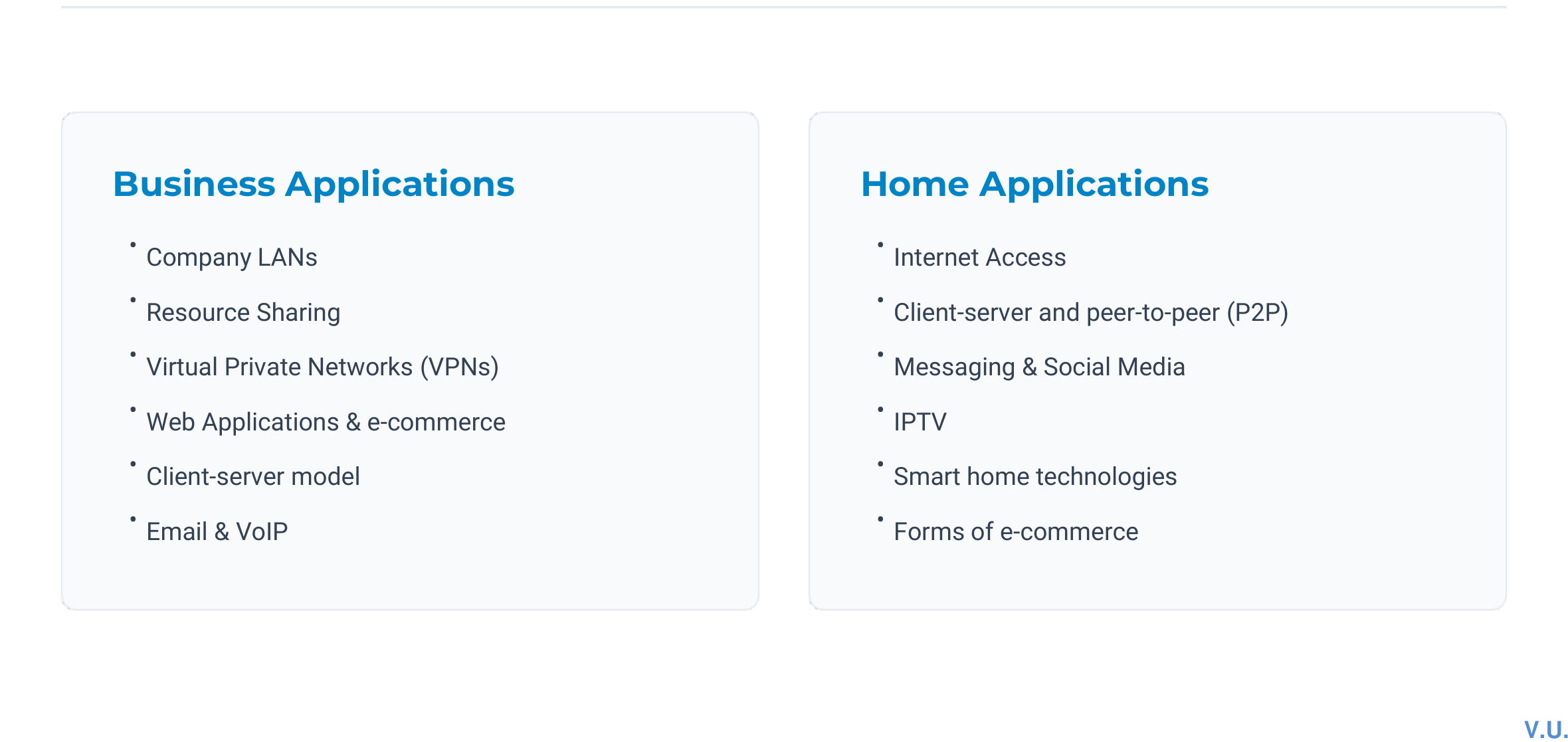
Business applications
Resource sharing: printers, storage, databases, and applications.
Client-server systems for web, email, enterprise software, and cloud services.
Remote access through virtual private networks.
Communication using email, messaging, voice, and video.
Home applications
Internet access and information retrieval.
Peer-to-peer communication and file exchange.
Streaming, social media, online learning, and e-commerce.
Smart-home services and connected devices.
Mobile applications
Cellular data, Wi-Fi hotspots, GPS navigation, and mobile commerce.
Wearables and sensor networks.
Connectivity while the user or device changes location.
Uses of computer networks grouped into business and home applications.
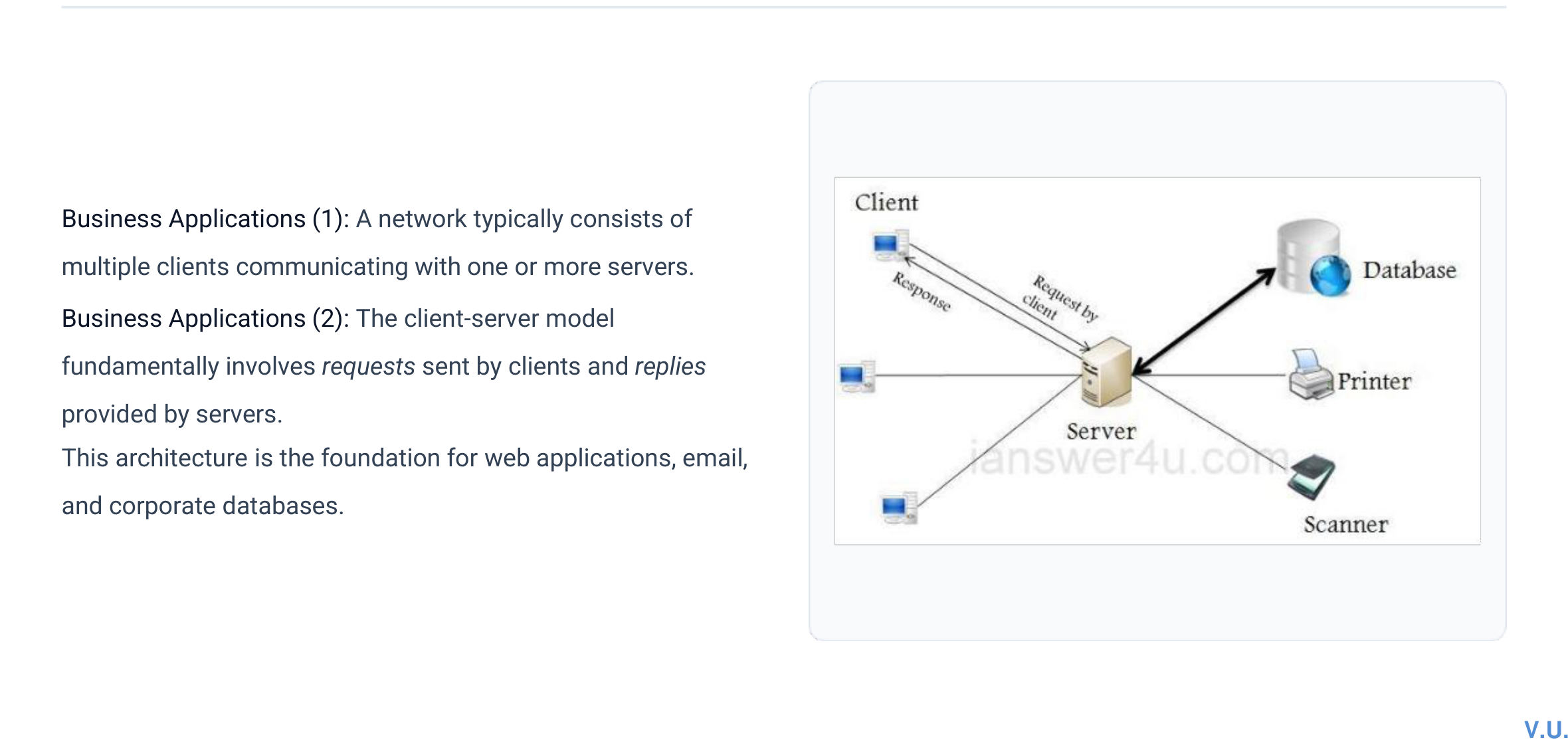
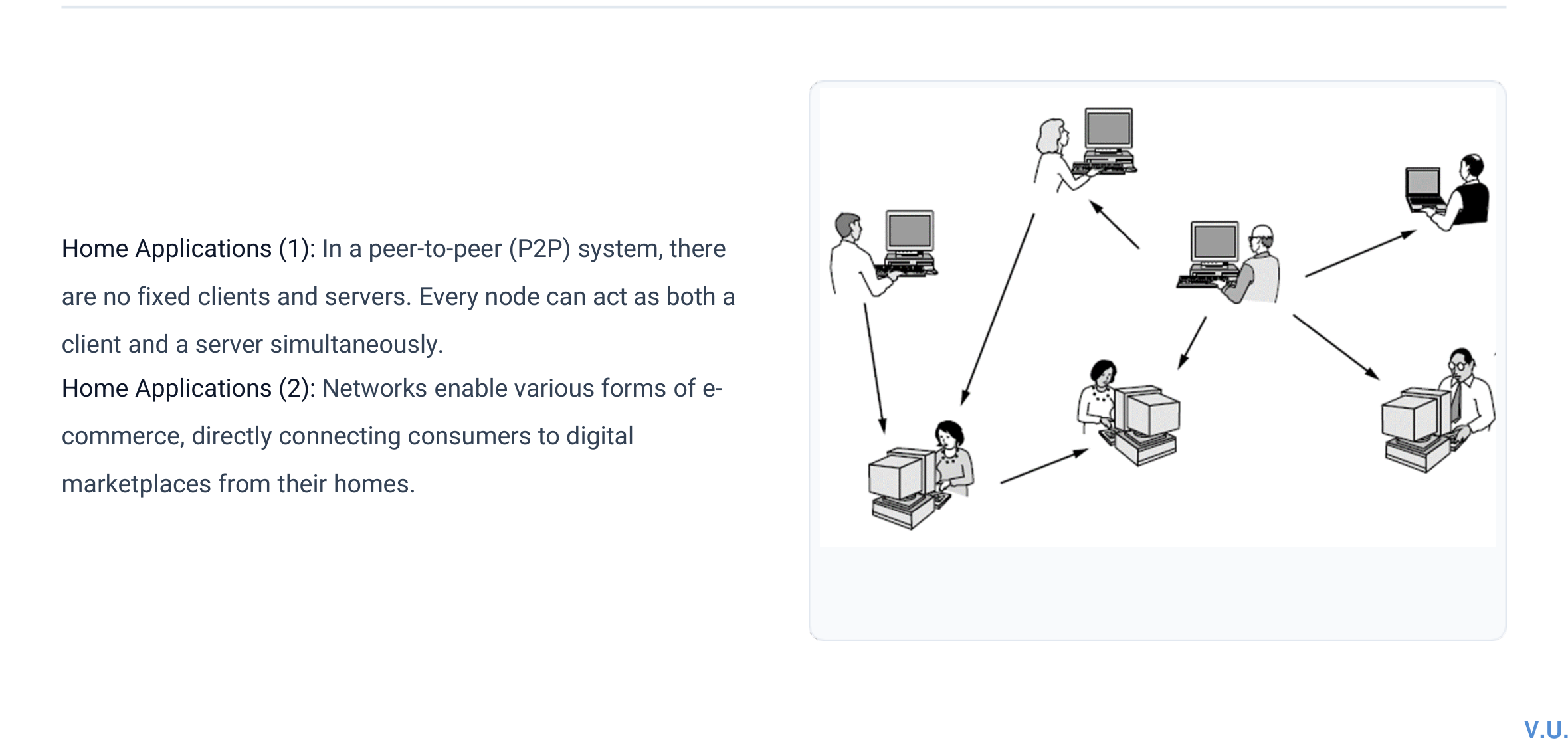
Client-server model: clients initiate requests; servers provide shared services.Peer-to-peer model: each peer can request and provide resources.
Client-server versus peer-to-peer
Aspect
Client-server
Peer-to-peer
Control
Centralized service and administration
Distributed among peers
Scalability
Server capacity can become a bottleneck
Resources may grow with peers, but coordination becomes harder
Security
Policies are easier to enforce centrally
Trust and consistency are harder to manage
Example
Web application and database server
Direct file sharing
Exam focus
Define a computer network, list business/home/mobile uses, and distinguish client-server from peer-to-peer architecture.
Quick revision
Networks enable communication and resource sharing.
Client-server centralizes service; peer-to-peer distributes it.
Mobile networking adds location change, wireless access, and mobility management.
1.2
Network Hardware: PAN, LAN, MAN, WAN, and the Internet
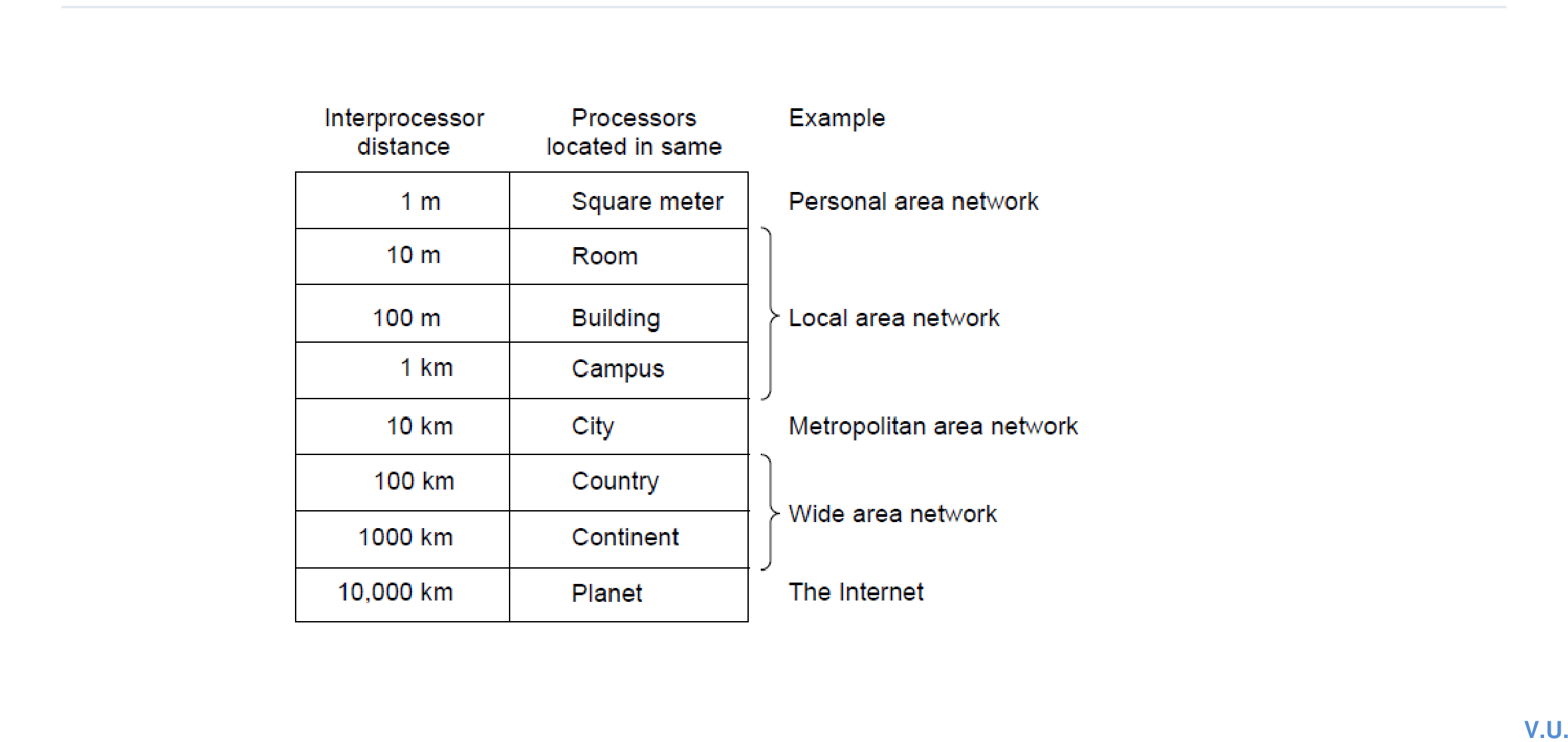
Network hardware is commonly classified by transmission technology and geographical scale. A broadcast link is shared by many devices; a point-to-point link directly connects a pair of devices. Delivery may be unicast, multicast, broadcast, or anycast.
Classification by scale: personal, local, metropolitan, wide-area, and global networks.
Network
Typical scope
Ownership / purpose
Typical example
PAN
A few metres around a person
Personal device interconnection
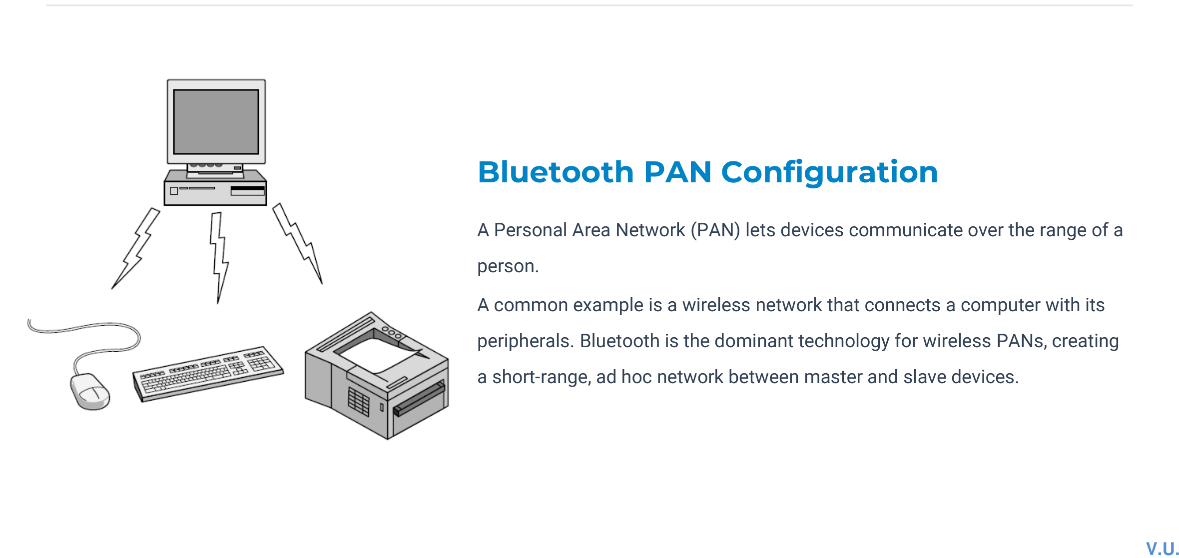
Bluetooth peripherals
LAN
Room, building, or campus
Usually privately owned; high data rate
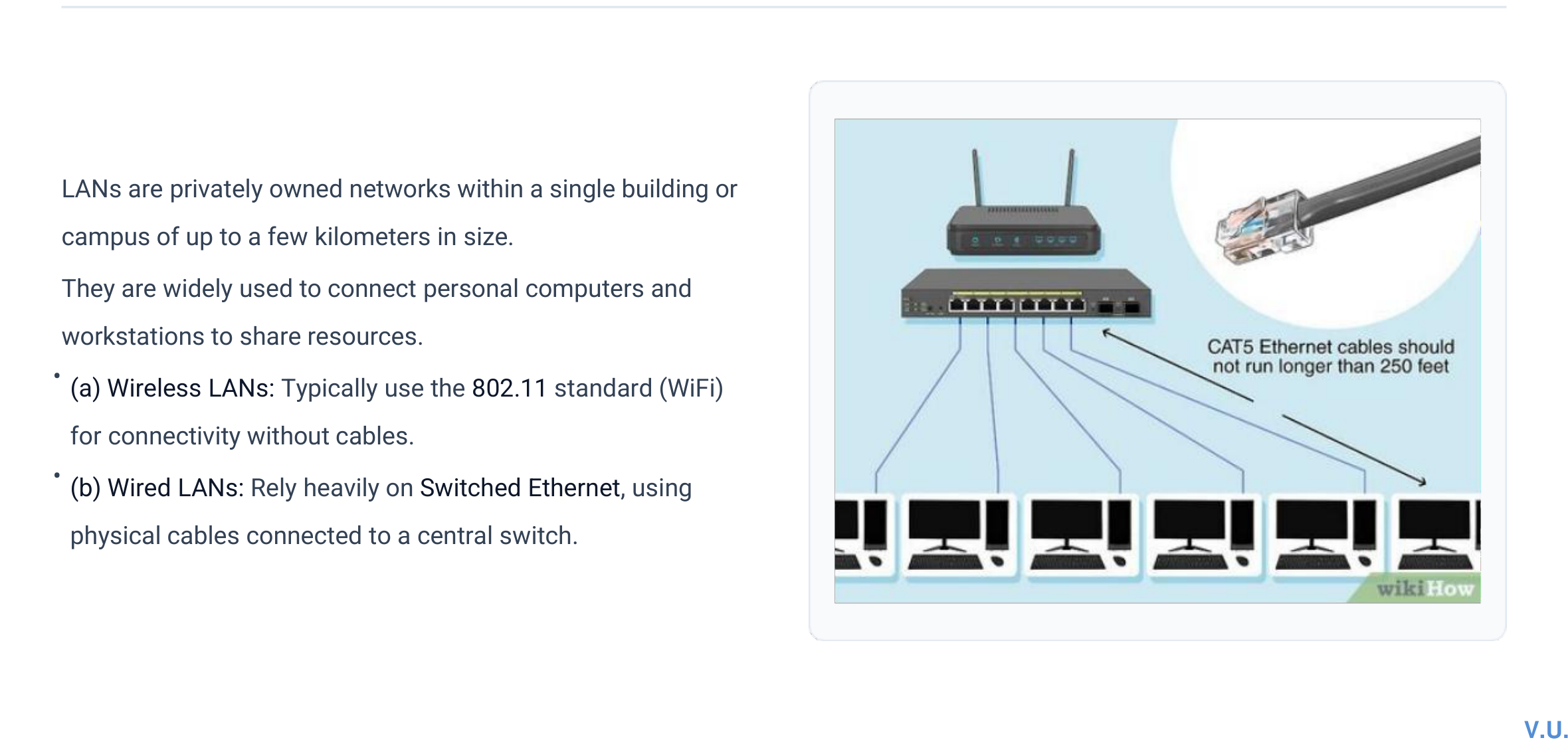
Office Ethernet or Wi-Fi
MAN
City or metropolitan area
Connects sites across a city
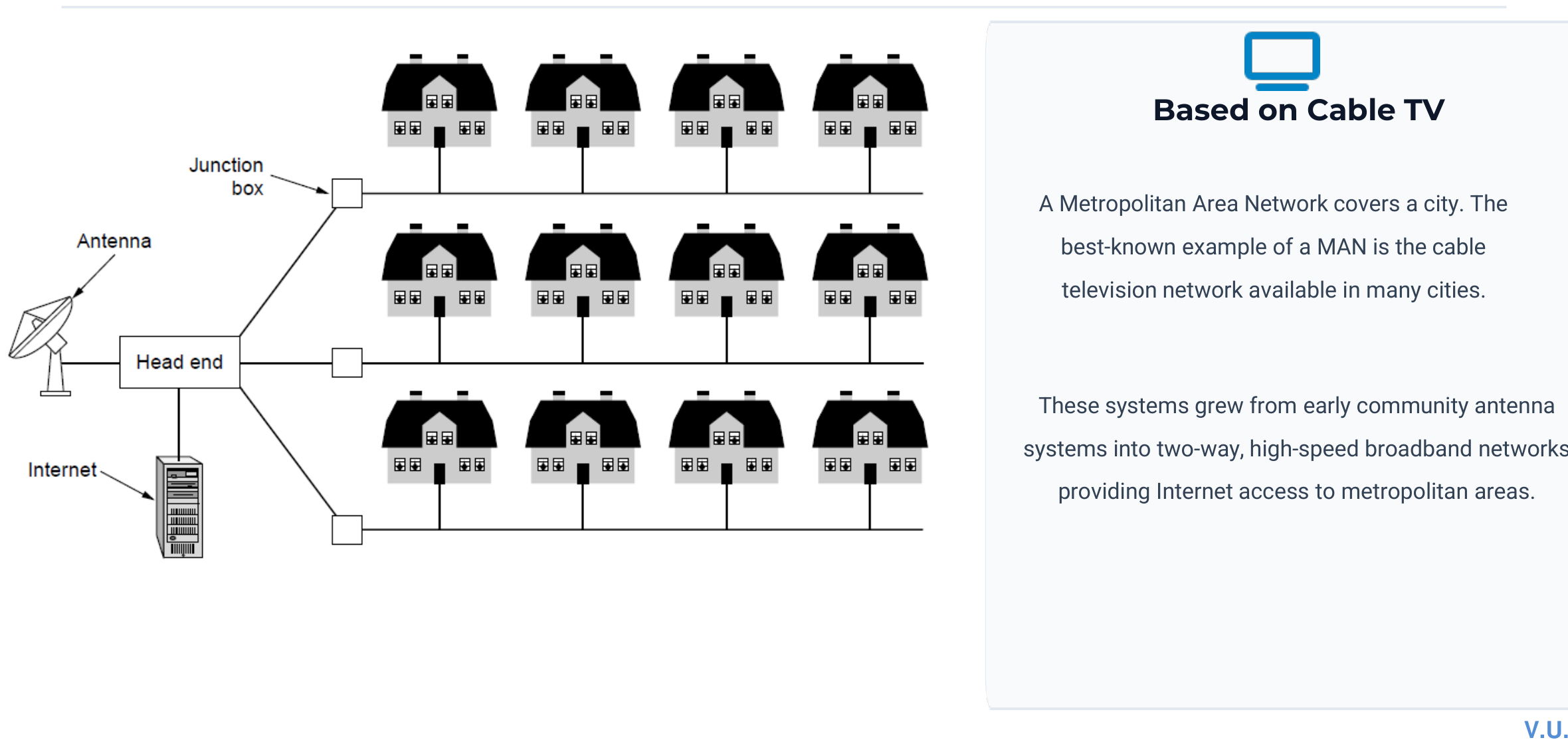
Metro Ethernet or cable network
WAN
Country or continent
Long-distance interconnection using carrier links
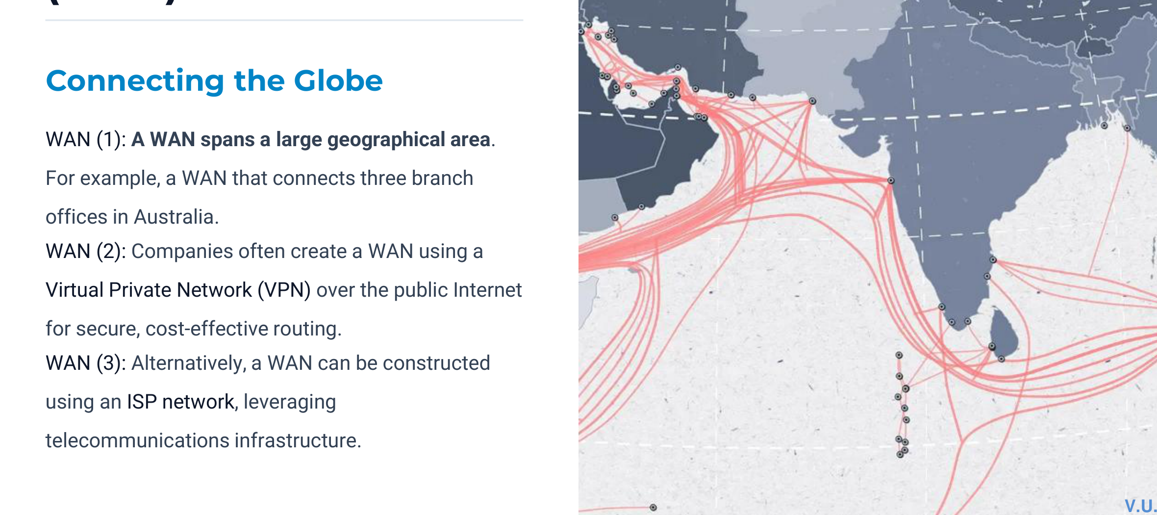
Enterprise branch network
Internet
Global
Interconnection of independently administered networks
The public Internet
PANLANMANWAN
Internet as a network of networks
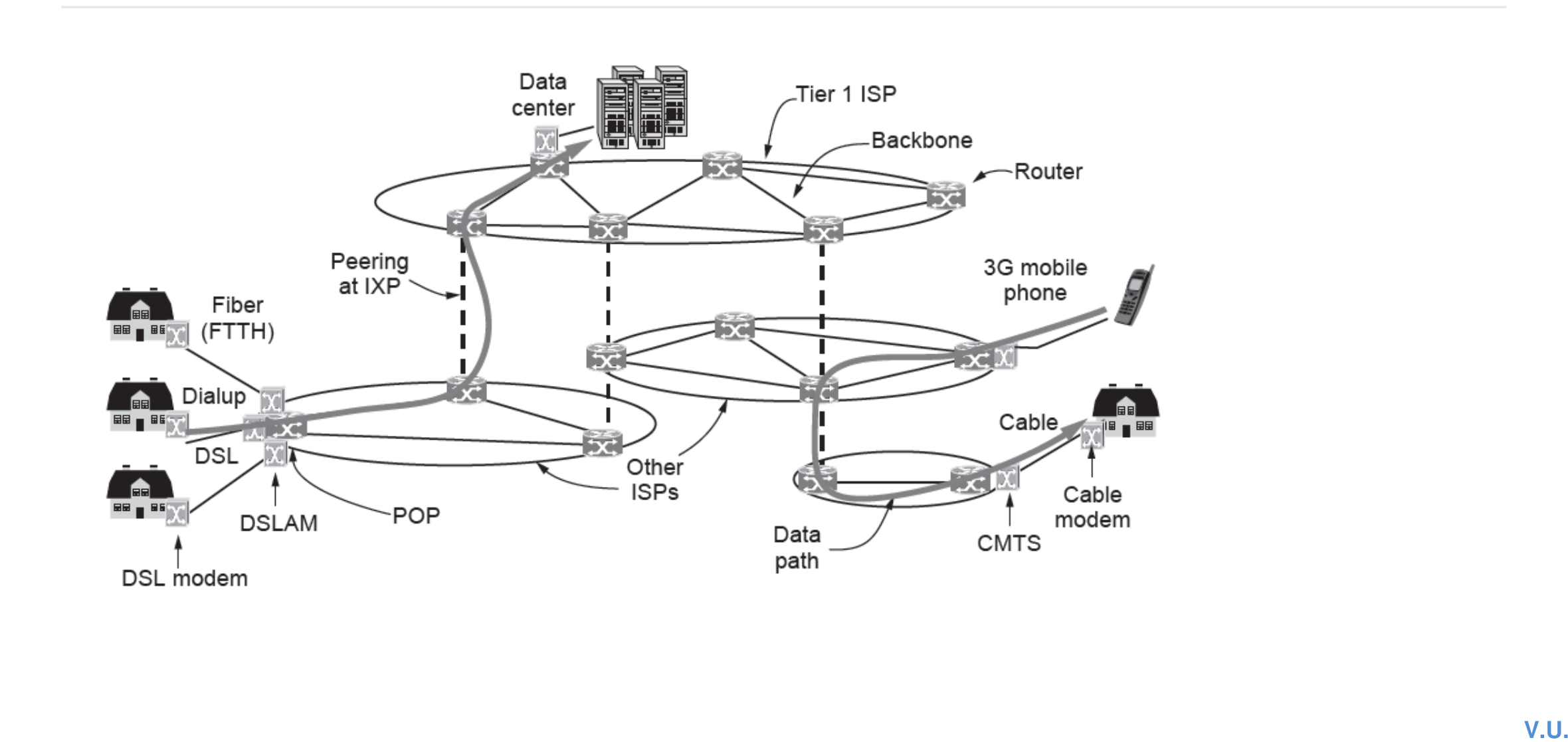
The Internet does not use one single owner or one physical technology. Internet service providers, enterprise networks, access networks, data centres, and backbone networks exchange packets using the TCP/IP protocol suite. Routers connect networks and choose packet paths.
Worked numerical: bits in a cable
Problem: A 1000 km cable operates at 1 Mbps. Propagation speed is 2/3 of the speed of light. How many bits fit in the cable?
Source: CN_Numericals_Data_Communication.pdf and Tutorial 3.
Quick revision
PAN → person, LAN → building/campus, MAN → city, WAN → large geographical region.
The Internet joins heterogeneous networks using routers and TCP/IP.
Bits in flight = data rate × propagation delay.
1.3
Network Software and Protocol Hierarchies
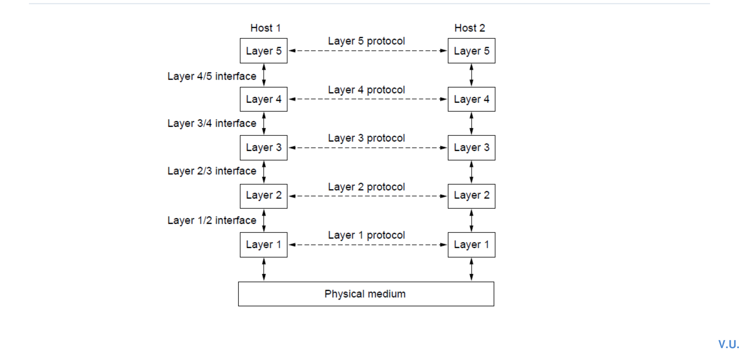
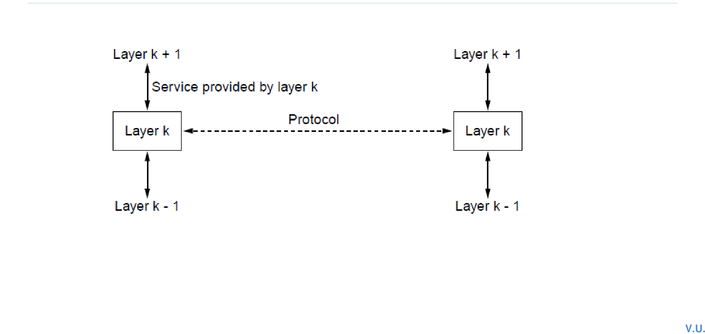
Network software is organized into layers. Each layer performs a related set of functions, offers services to the layer above it, and uses services of the layer below it. A protocol specifies the rules and formats used by peer entities in the same layer; an interface defines how adjacent layers interact.
Protocols act horizontally between logical peers; interfaces act vertically between neighbouring layers.
Why layering is used
Reduces design complexity by separating concerns.
Allows a layer implementation to change without redesigning every other layer, provided its service interface remains stable.
Promotes interoperability and standardization.
Makes testing, troubleshooting, and protocol evolution easier.
Encapsulation and virtual communication
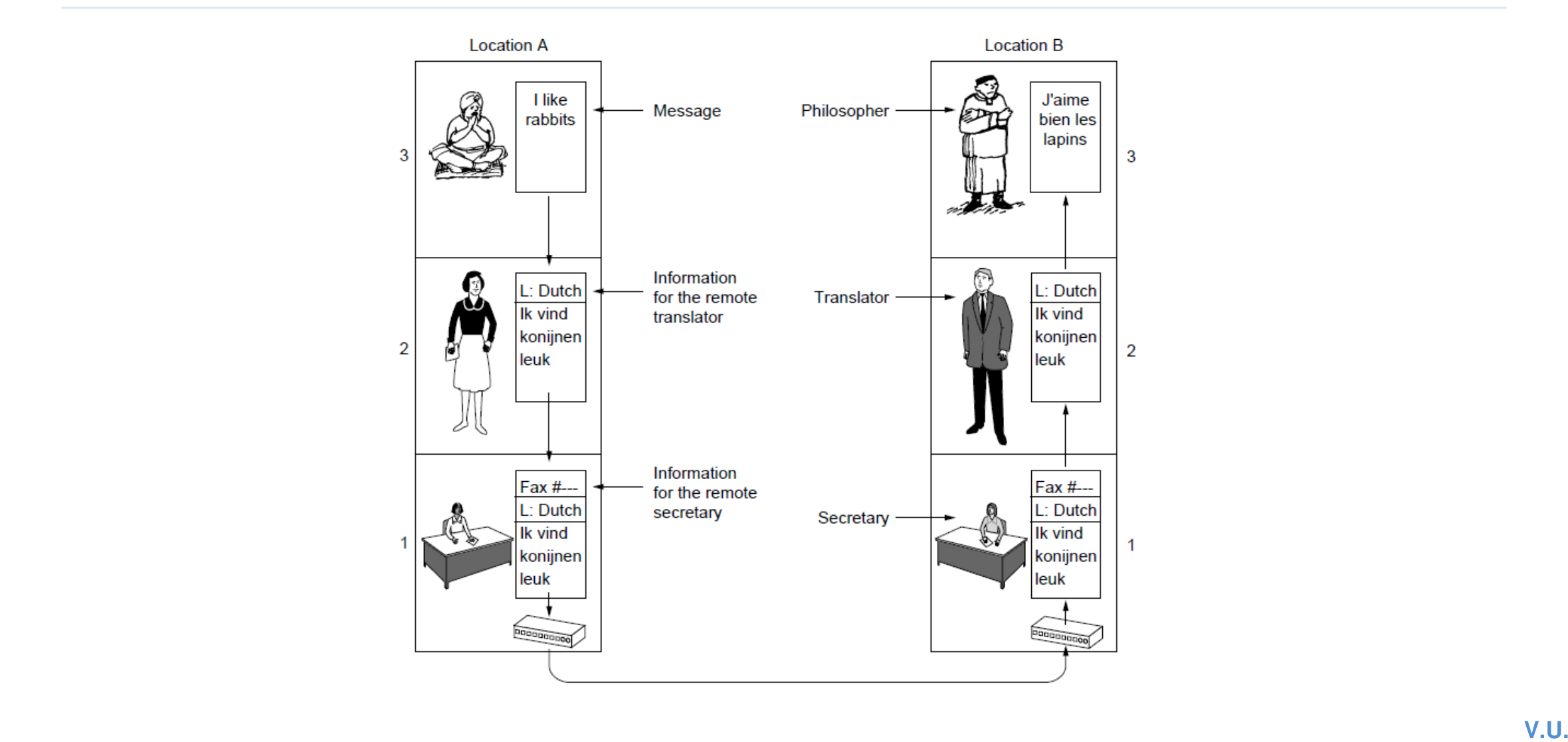
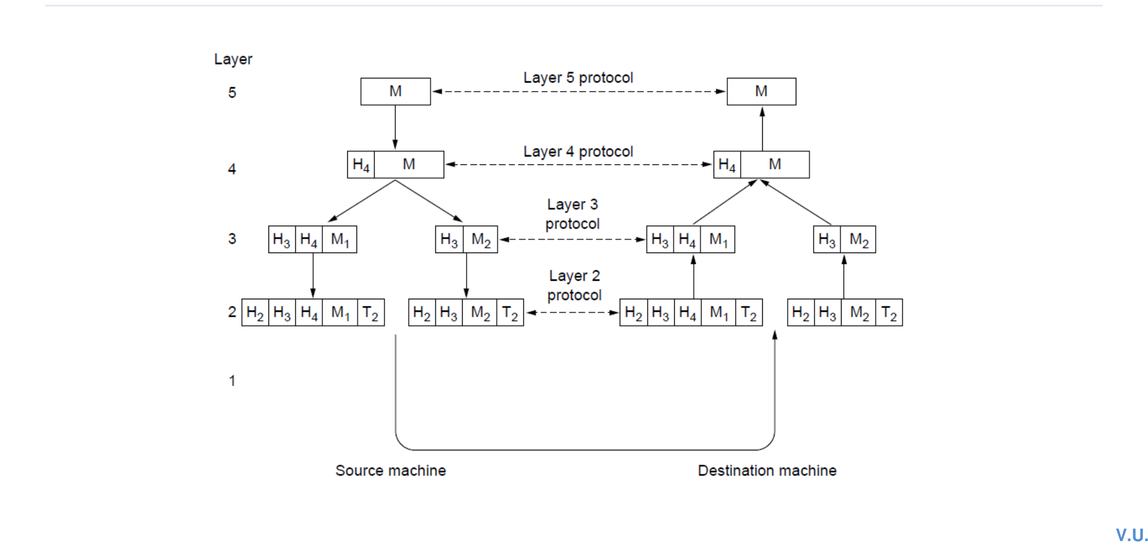
When data moves downward, each layer may add control information called a header (and sometimes a trailer), creating its protocol data unit. At the receiver, the process is reversed. Peer layers appear to communicate directly, but actual bits travel through lower layers and the physical medium.
The philosopher-translator-secretary analogy separates logical peer communication from physical delivery.Each layer treats the lower-layer path as a virtual channel to its peer.
Three terms that must not be mixed
Service: what a layer provides.
Interface: how the service is accessed.
Protocol: how peer entities cooperate to provide it.
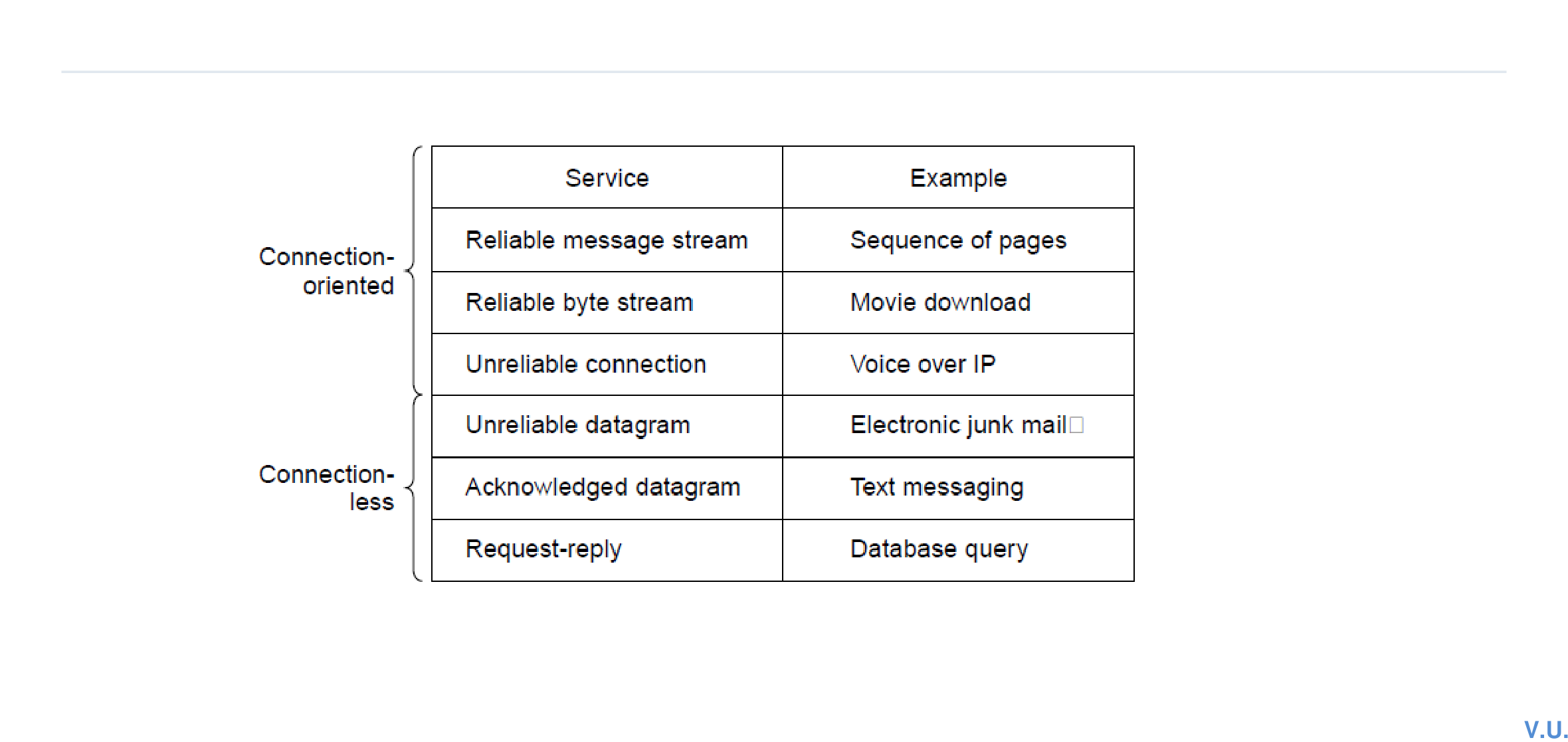
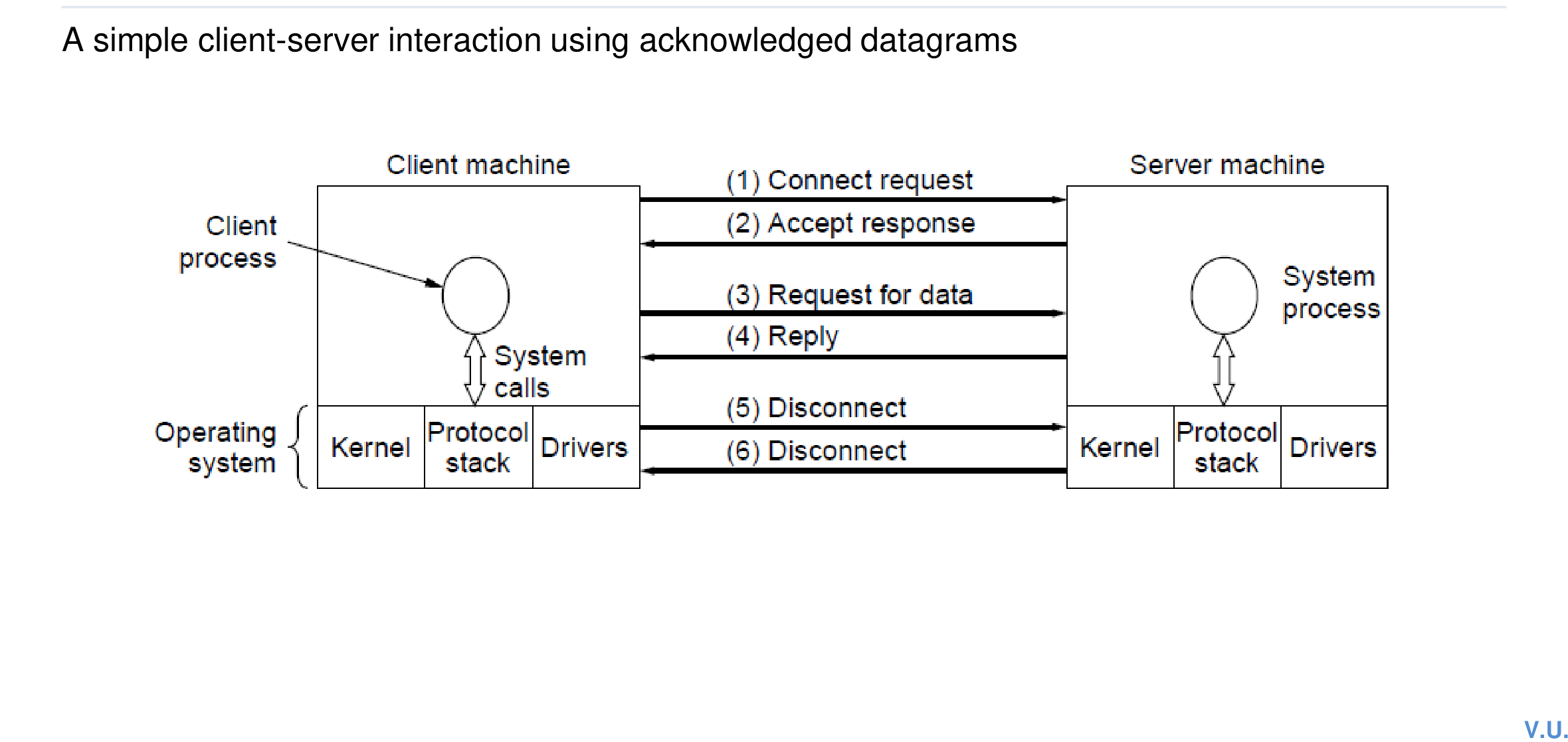
A service describes the behaviour visible to the service user. It may be connection-oriented, where state is established before transfer, or connectionless, where each message is treated independently.
Both service families can be reliable or unreliable depending on the contract provided.
Aspect
Connection-oriented
Connectionless
Setup
Connection established before data transfer
No prior setup
State
Endpoints or network maintain connection state
Each message carries enough information to be handled independently
Ordering
Often preserves order
Messages may take different paths or arrive out of order
Connection-oriented does not automatically mean reliable, and connectionless does not automatically mean unreliable. Reliability is a separate property of the service contract.
Quick revision
Connection-oriented service usually has setup, transfer, and release phases.
Connectionless service handles messages independently.
Reliability and connection style are independent dimensions.
1.6
Service Primitives and the Relationship of Services to Protocols
A service is accessed through operations called service primitives. A simple connection-oriented interface may use LISTEN, CONNECT, RECEIVE, SEND, and DISCONNECT.
Primitive
Purpose
LISTEN
Wait for an incoming connection.
CONNECT
Actively establish a connection with a peer.
RECEIVE
Wait for or obtain incoming data.
SEND
Transfer data to the peer.
DISCONNECT
Release the connection.
Service primitives describe the operations visible at the interface.A layer provides a service upward while using a protocol to cooperate with its peer.
Key relationship
Services define what operations a layer offers. Protocols define how peer entities exchange messages to implement those services. A service can remain unchanged even if its underlying protocol is replaced.
Quick revision
Primitives are interface operations.
A protocol is hidden behind the service interface.
Do not describe LISTEN or SEND as layers; they are service operations.
1.7
OSI Reference Model
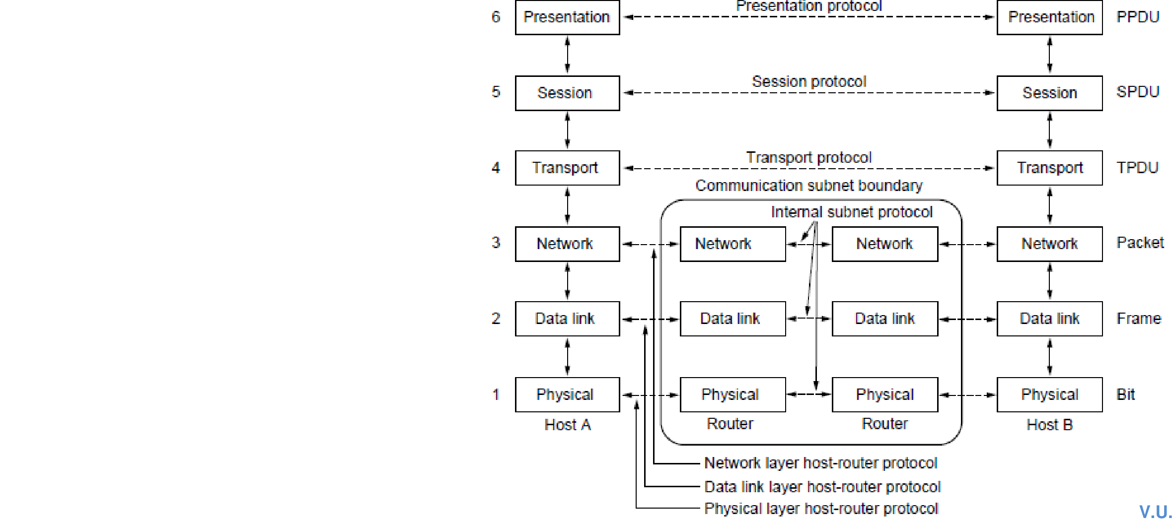
The ISO Open Systems Interconnection model organizes networking into seven conceptual layers. It is primarily a reference and teaching model: each layer groups well-defined functions and communicates through interfaces.
OSI layers and their peer-to-peer logical communication.
Layer
Primary responsibility
Typical unit
7 Application
Network services for user applications
Data / message
6 Presentation
Data representation, translation, compression, encryption
Data
5 Session
Dialogue management, synchronization, checkpoints
Data
4 Transport
End-to-end delivery, segmentation, reliability, flow control
Segment
3 Network
Logical addressing and routing
Packet
2 Data Link
Framing, MAC addressing, link reliability
Frame
1 Physical
Raw bit transmission and signal characteristics
Bit
Exam focus
Long answers usually require the seven layers in order, the responsibility of each layer, and the distinction between end-to-end (transport) and hop-to-hop/link-local (data link) operation.
Quick revision
OSI has seven layers.
Network routes packets; data link carries frames across one link.
Transport provides process-to-process end-to-end service.
1.8
TCP/IP Reference Model
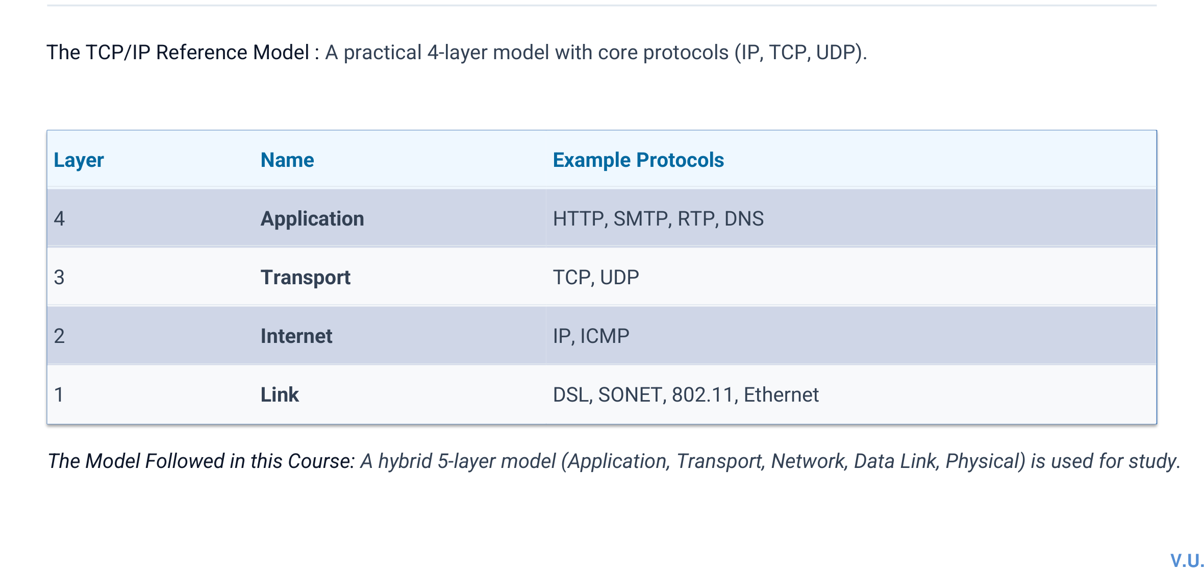
The TCP/IP model grew from operational internetworking and the ARPANET. In the four-layer version used by the course, the layers are Link, Internet, Transport, and Application.
TCP/IP layers and representative protocols.
TCP/IP layer
Role
Examples
Application
Application protocols and data formats
HTTP, SMTP, DNS
Transport
End-to-end process communication
TCP, UDP
Internet
Best-effort packet delivery across networks
IP, ICMP
Link
Local delivery over the attached network
Ethernet, Wi-Fi, PPP
IP provides an unreliable best-effort datagram service. Reliability, ordering, and congestion/flow functions may be added at the transport layer by TCP. UDP provides a lighter connectionless transport service.
Quick revision
TCP/IP is the practical architecture of the Internet.
IP is at the Internet layer; TCP and UDP are transport protocols.
Application protocols use transport services.
1.9
Comparison and Critique of OSI and TCP/IP
Dimension
OSI
TCP/IP
Origin
Reference model designed before its protocol suite matured
Model abstracted from working protocols and operational networks
Layers
Seven
Usually four (sometimes shown as five)
Service/interface/protocol distinction
Explicit and conceptually clear
Less sharply separated in the original model
Network service
Could describe connection-oriented and connectionless approaches
Internet layer is connectionless; reliability mainly belongs to transport
Adoption
Widely used for teaching and analysis
Dominant deployed Internet protocol architecture
Critique of OSI
Bad timing: the protocol suite competed with already-growing TCP/IP deployment.
Bad technology: some functions and layer boundaries were considered complex or awkward.
Bad implementations: early implementations were large and slow.
Bad politics: TCP/IP was associated with open academic/Internet growth while OSI was perceived as committee-driven.
Critique of TCP/IP
The model does not cleanly distinguish services, interfaces, and protocols.
The host-to-network/link layer is underspecified.
It is less general as a reference model because it closely follows one protocol suite.
Some layer functions are not separated as cleanly as in OSI.
Key takeaway
OSI is stronger as a conceptual model; TCP/IP is stronger as a deployed architecture. In exams, avoid claiming that OSI “failed completely” or that TCP/IP has no model—it remains the basis of Internet protocol organization.
Quick revision
OSI: cleaner abstractions, seven layers.
TCP/IP: working protocol suite, four layers, global adoption.
Both use layering but draw boundaries differently.
1.10
Example Networks and Important Network Standards
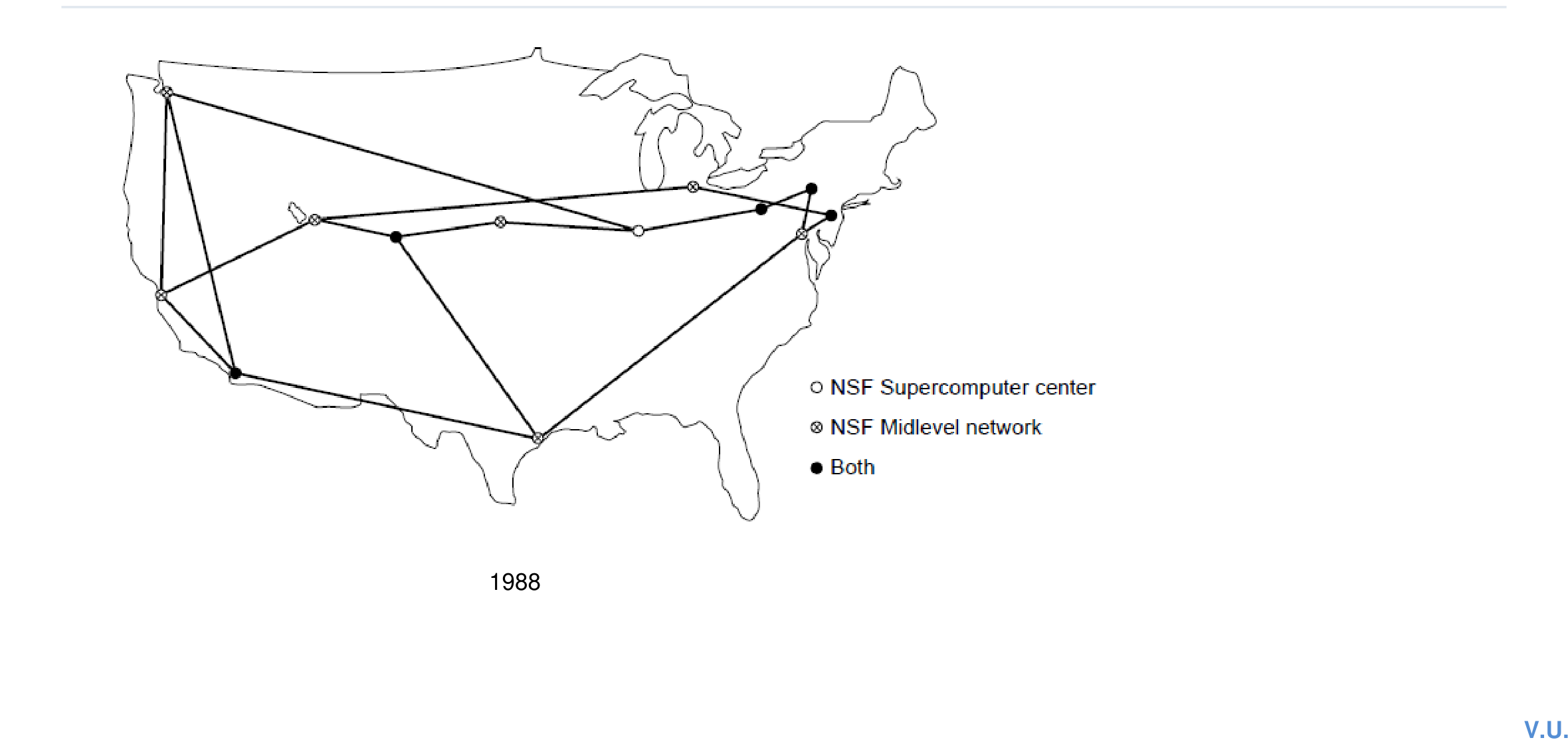
Example networks show how architectural ideas become real systems. ARPANET demonstrated packet switching and internetworking; NSFNET expanded academic backbone connectivity; the modern Internet is a hierarchy of access networks, regional providers, backbone providers, Internet exchange points, and data centres.
NSFNET expanded high-speed academic backbone connectivity.The Internet is an interconnection of many independently managed networks.
Why standards matter
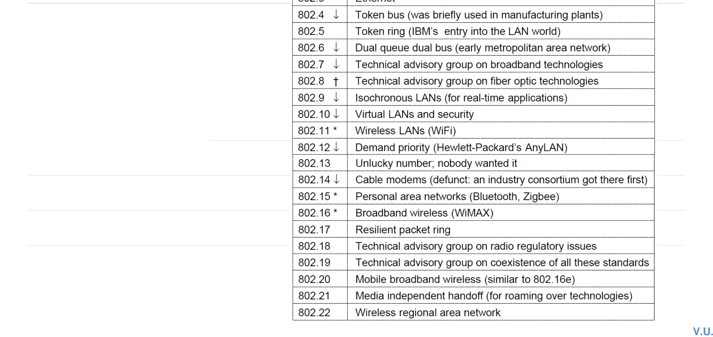
Standards let equipment and software from different vendors interoperate. De facto standards become accepted through widespread use; de jure standards are formally approved by recognized organizations.
Layered architecture, OSI stack, TCP/IP stack, network scale.
Numerical patterns
Propagation delay, bits in flight, Nyquist capacity, Shannon capacity.
03
Chapter 3
Data Link Layer
Services to the network layer, frame boundaries, flow control, elementary protocols, sliding windows, SONET, and ADSL.
3.1
Services Offered to the Network Layer
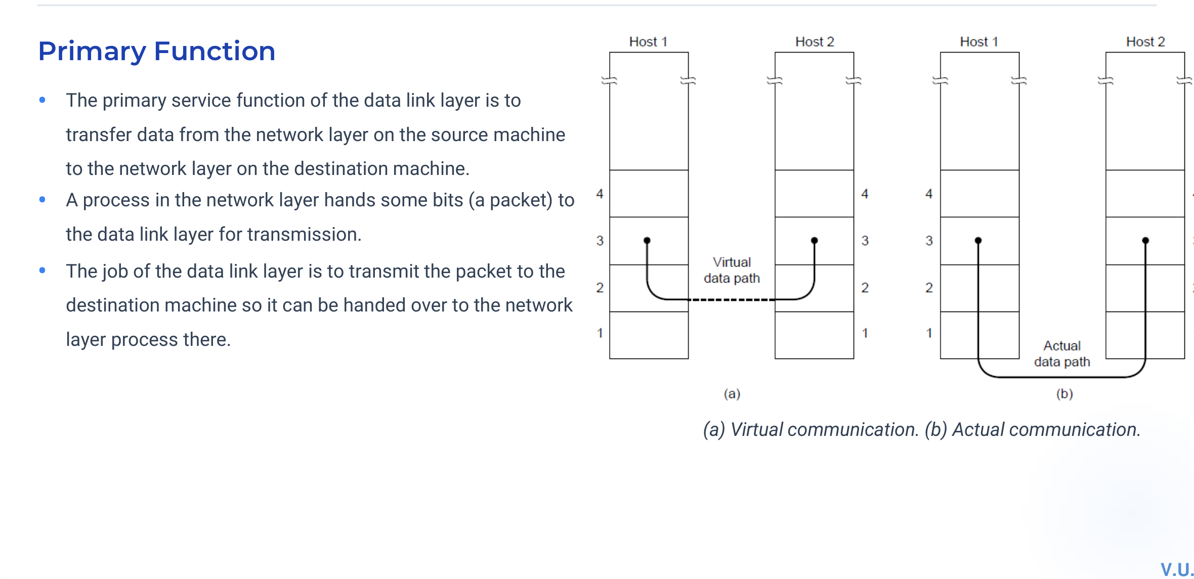
The data link layer converts the raw service of the physical layer into a link service for the network layer. It accepts packets, places them in frames, coordinates transmission over one link, and hands received packets upward.
The network layer sees a logical link service; actual data crosses the physical medium as frames and bits.
Service
Connection?
Acknowledgement?
Typical use
Unacknowledged connectionless
No
No
Reliable low-error links or time-sensitive traffic
Acknowledged connectionless
No
Each frame
Unreliable links where local recovery is useful
Acknowledged connection-oriented
Yes
Yes, with sequencing
Reliable ordered frame delivery
Scope note
The chapter explains reliable protocols, but error-control coding techniques such as CRC and Hamming code are excluded from this syllabus.
Quick revision
Packets are network-layer units; frames are data-link units.
Data-link services differ by connection state and acknowledgement behaviour.
Frame management is the layer's central job.
3.2
Framing
The physical layer supplies a continuous bit stream. Framing divides that stream into recognizable units so headers, payload, and trailer information can be interpreted correctly and the receiver can resynchronize after disturbances.
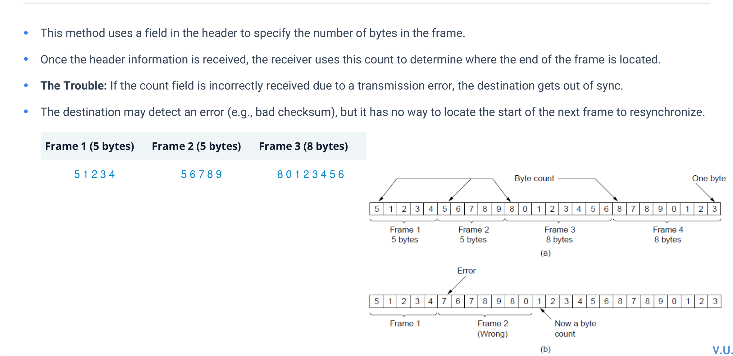
1. Byte count
A header field gives the frame length. The receiver counts that many bytes to find the next frame. Its weakness is loss of synchronization when the count field is corrupted.
A damaged count can make the receiver locate later frame boundaries incorrectly.
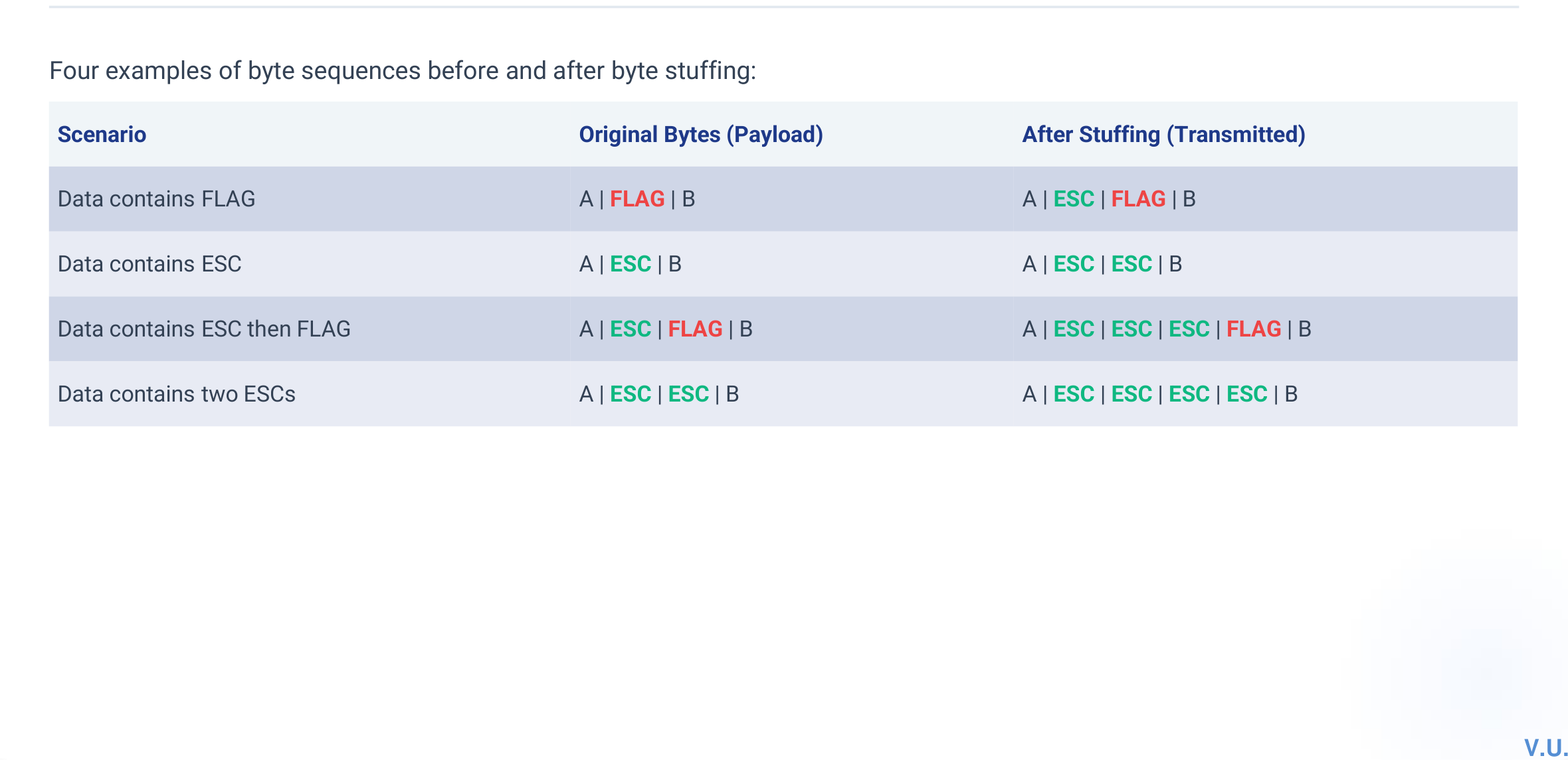
2. Flag bytes with byte stuffing
Special FLAG bytes mark the beginning and end. If FLAG or ESC occurs inside the data, the sender inserts ESC before it. The receiver removes the inserted ESC during destuffing.
Byte stuffing keeps payload bytes from being mistaken for delimiters.
Worked example: byte stuffing
Problem: Data fragment: A B ESC C ESC FLAG FLAG D. Find the stuffed data and complete frame.
Rule: Insert ESC before every data ESC and every data FLAG.
Stuffed data:A B ESC ESC C ESC ESC ESC FLAG ESC FLAG D
Complete frame:FLAG A B ESC ESC C ESC ESC ESC FLAG ESC FLAG D FLAG
Source: CN_Numericals_Data_Link_Layer.pdf and Tutorial 1.
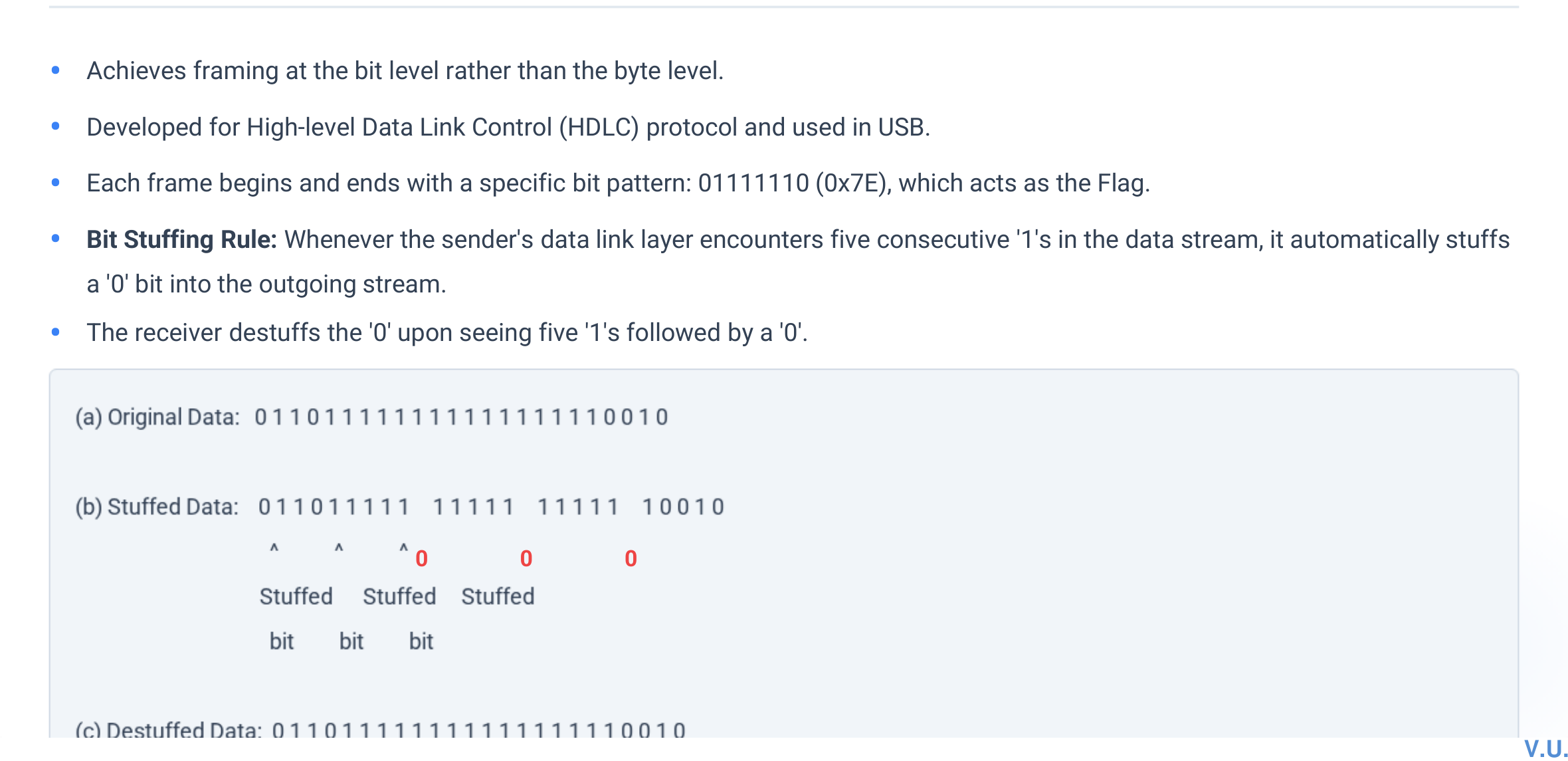
3. Flag bits with bit stuffing
A bit pattern, commonly 01111110, acts as a flag. After five consecutive 1s in payload data, the sender inserts a 0. The receiver removes that 0. Thus the flag pattern cannot appear unintentionally inside data.
Inserted zeros are protocol overhead and are removed by the receiver.
Worked example: bit stuffing
Problem: Stuff 0111101111101111110.
Scan: insert a 0 after every run of five 1s.
Final transmitted data:011110111110011111010.
Verified against CN_Numericals_Data_Link_Layer.pdf and Tutorial 1.
4. Physical-layer coding violations
Some line codes reserve signal patterns that cannot appear in valid encoded data. A data-link protocol can use those illegal patterns as unambiguous frame boundaries without byte or bit stuffing.
Method
Boundary mechanism
Main weakness / requirement
Byte count
Length field
Corrupted count destroys synchronization
Byte stuffing
FLAG byte
Byte-oriented; extra ESC overhead
Bit stuffing
Flag bit pattern
Bit scanning and stuffed-bit overhead
Coding violation
Unused physical signal
Requires a line code with invalid/reserved symbols
Quick revision
Framing provides boundaries and synchronization.
Stuffing makes delimiter values transparent to payload data.
Byte count is simple but vulnerable to a corrupted length field.
3.3
Flow Control
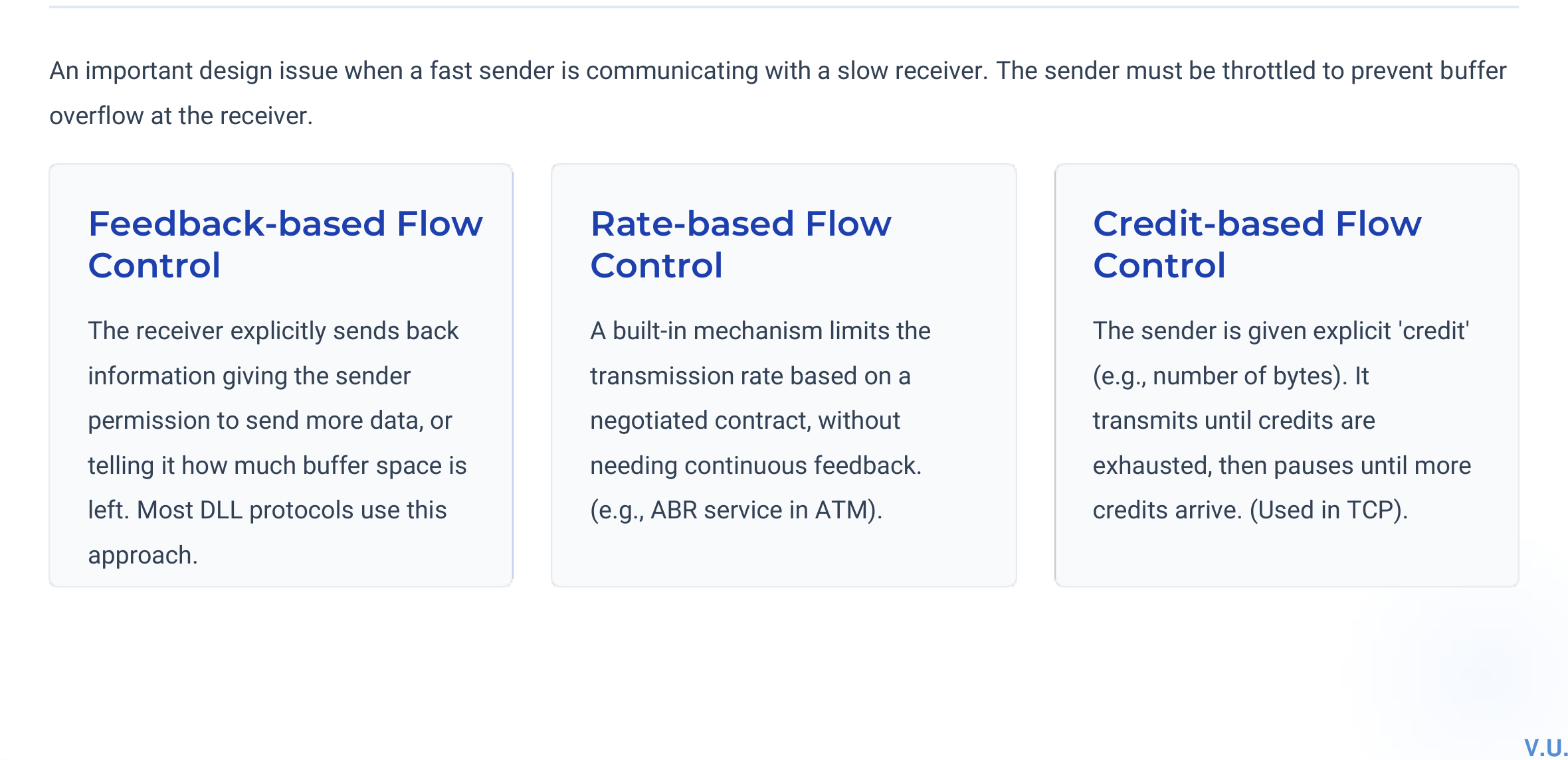
Flow control prevents a fast sender from delivering frames faster than a receiver can accept, buffer, and process them. It concerns receiver capacity; it must not be confused with congestion control, which concerns overload inside the network.
Three ways to constrain the sender: explicit feedback, an agreed rate, or receiver-issued credits.
Feedback-based
The receiver sends information telling the sender when or how much to send. Stop-and-wait and sliding-window acknowledgements are examples.
Rate-based
The sender is limited to an agreed average or peak rate without requiring continuous per-frame feedback.
Credit-based
The receiver grants credits representing available buffer space. Sending consumes credits; new credits reopen capacity.
Key distinction
Flow control answers “Can the receiver keep up?” Congestion control answers “Can the network carry the offered load?”
Quick revision
Feedback reacts to receiver information.
Rate control limits long-term sending speed.
Credit control directly represents available receiving capacity.
3.4
Elementary Data Link Protocols
Utopian simplex protocol
Assumes data travels in one direction, the channel never damages or loses frames, the receiver is always ready, and its buffer is unlimited. The sender repeatedly obtains a packet, places it in a frame, and transmits. It is a baseline rather than a practical protocol.
Simplex stop-and-wait for an error-free channel
Removes the assumption of an infinitely fast receiver. The sender transmits one frame and waits for an acknowledgement before taking the next packet. This provides feedback-based flow control but wastes capacity on long-delay links.
Simplex stop-and-wait for a noisy channel
Adds sequence numbers, acknowledgements, a timer, and retransmission. If a data frame or ACK is lost, the sender eventually times out and sends again. A one-bit sequence number is sufficient because only one frame can be outstanding; it lets the receiver detect duplicates.
Sender gets a packet and builds the next numbered frame.
Sender transmits and starts a timer.
Receiver accepts an undamaged expected frame, delivers it once, and returns an ACK.
Correct ACK arrives → advance the sequence number.
Timeout → retransmit; duplicate data is acknowledged but not delivered twice.
Worked numerical: stop-and-wait transfer time
Problem: Each packet carries 1000 data bits. Send 1,000,000 bits over 5000 km at propagation speed 2 × 10⁸ m/s. Ignore transmission and processing delays.
Noisy stop-and-wait adds timer, ACK, retransmission, and a one-bit sequence number.
3.5
Sliding Window and One-Bit Sliding Window Protocol
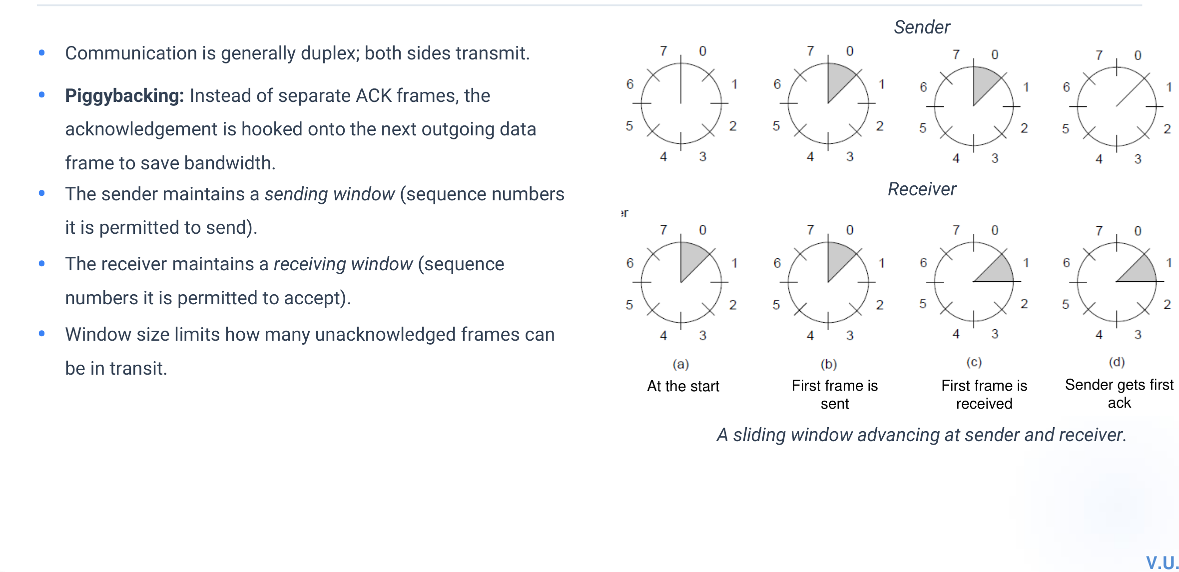
A sliding-window protocol allows sequence numbers within a moving range. The sender window contains frames that may be transmitted or are awaiting acknowledgement; the receiver window contains sequence numbers it is prepared to accept.
Windows move as frames are sent, received, and acknowledged.
Piggybacking
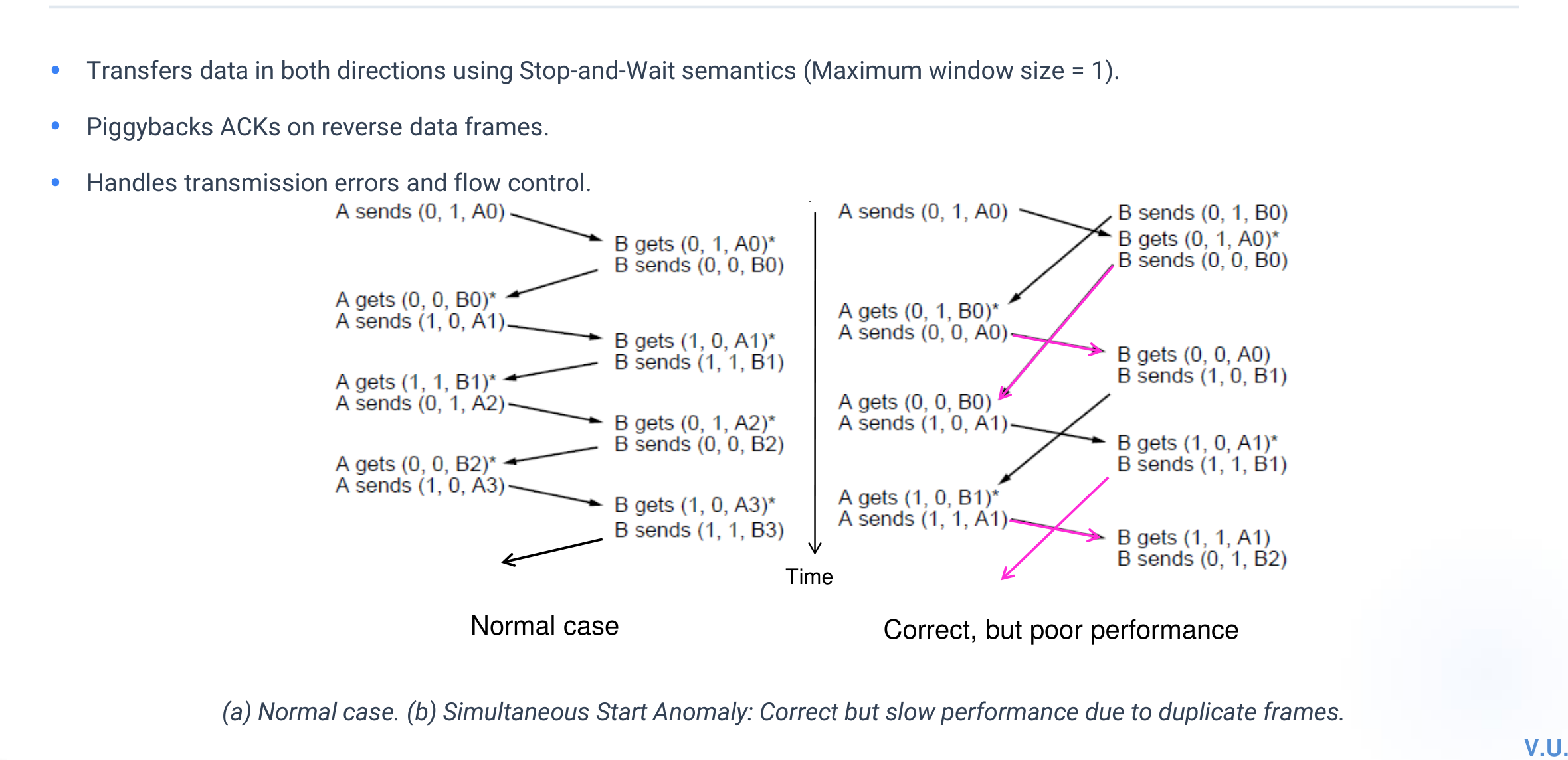
On a full-duplex link, an acknowledgement can be carried in the header of a reverse-direction data frame rather than sent separately. A short timer prevents an ACK from being delayed indefinitely when reverse traffic is absent.
One-bit sliding window
With sequence numbers 0 and 1 and maximum window size 1, both sides alternate expected numbers. This is essentially bidirectional stop-and-wait with piggybacking. Duplicate frames are recognized by the sequence bit.
Alternating sequence bits prevent a retransmission from being delivered as new data.
Stop-and-wait utilization
U = 1 / (1 + 2a), where a = Tprop / Ttrans, when ACK transmission and processing are negligible.
Worked numerical: window for full utilization
Problem: Earth-to-planet distance = 9 × 10¹⁰ m, rate = 64 Mbit/s, frame = 32 kB, propagation speed = 3 × 10⁸ m/s. Find the sender window for 100% utilization.
One-way delay: 300 s. Frame transmission: 262,144/(64 × 106) = 0.004096 s.
a: 300/0.004096 ≈ 73,242. Full utilization requires W ≥ 1 + 2a ≈ 146,485 frames.
Course-material answer: 150001, using 32 kB ≈ 256 kbit and Ttrans = 0.004 s. Verified exact binary-kilobyte result: approximately 146485. Both use the same formula; the difference is unit rounding.
Quick revision
Windows permit multiple outstanding frames.
Piggybacking combines data and ACK information.
One-bit sliding window is stop-and-wait in both directions.
3.6
Go-Back-N
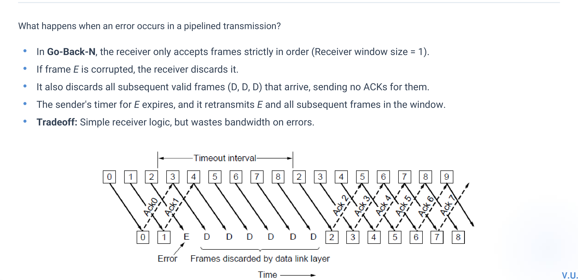
Go-Back-N pipelines frames. The sender may have up to W unacknowledged frames, while the receiver window is 1. The receiver accepts only the next expected frame and discards later out-of-order frames. ACKs are cumulative.
When a frame is missing, later frames are discarded and the sender retransmits from the missing frame onward.
Window-size rule
For an m-bit sequence number, Go-Back-N normally uses a sender window no larger than 2m − 1. Reserving one sequence number prevents an old frame from being confused with a new frame after wraparound.
Worked numerical: sequence-number bits
Problem: A 3000 km T1 trunk sends 64-byte frames. Propagation is 6 μs/km. How many sequence-number bits keep the pipe full?
Propagation: 18 ms one way; ACK returns after roughly 36 ms.
Frame transmission: 512/1.536 Mbit/s ≈ 0.333 ms.
Outstanding frames: about 36.33/0.333 ≈ 109; therefore at least 110 sequence positions are useful.
Final answer: 7 bits (128 sequence values). The course slide approximates 0.300 ms and 121 frames; the bit-width conclusion is unchanged.
Worked example: window after damage
A uses W = 7 and 3-bit sequence numbers. Frames 0–6 are sent; frame 4 is damaged. The sender's next window after earlier cumulative acknowledgements advances modulo 8.
Course answer: 4, 5, 6, 7, 0, 1, 2.
Source: CN_Numericals_Data_Link_Layer.pdf and Tutorial 2.
Quick revision
Receiver window = 1.
ACKs are cumulative.
An error can cause many correct later frames to be retransmitted.
3.7
Selective Repeat
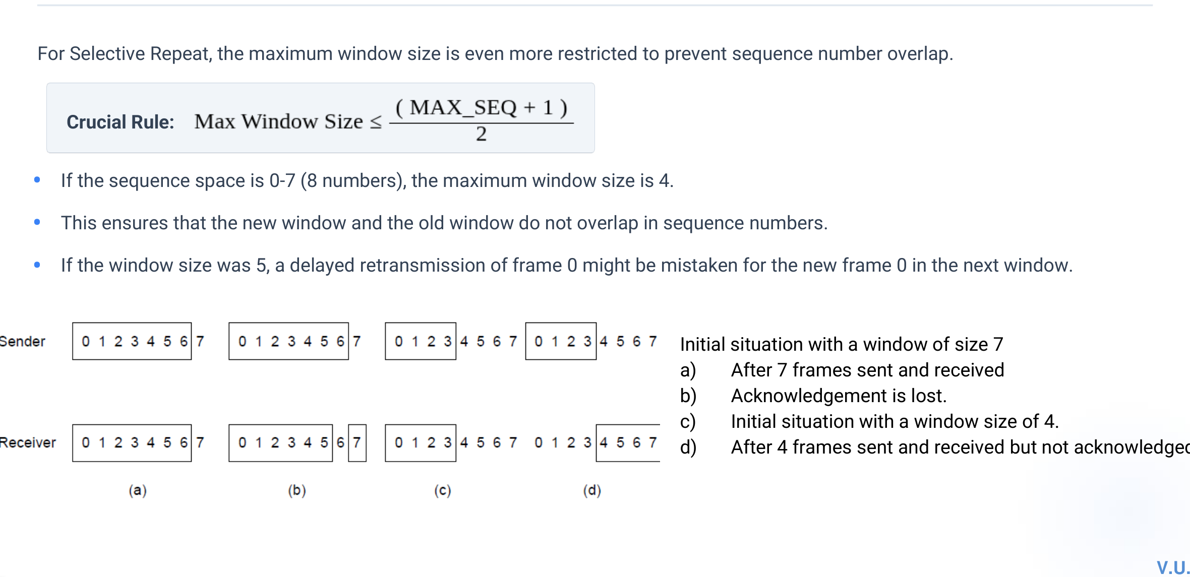
Selective Repeat retransmits only frames that are lost or damaged. The receiver accepts and buffers valid out-of-order frames, acknowledges them individually, and delivers them upward after the missing gap is filled.
Sender and receiver windows must not overlap old and new interpretations of the same sequence number.
Aspect
Go-Back-N
Selective Repeat
Receiver window
1
Greater than 1
Out-of-order frames
Discarded
Buffered
Retransmission
Missing frame and later outstanding frames
Only missing/damaged frame
Receiver complexity
Lower
Higher
Bandwidth on noisy links
May be wasted
More efficient
Window limit
With m sequence bits, sequence space S = 2m. For Selective Repeat, sender and receiver window sizes must normally satisfy W ≤ S/2 = 2m−1.
Common mistake
Using a Selective Repeat window larger than half the sequence space can make an old delayed frame indistinguishable from a new frame with the same wrapped sequence number.
Quick revision
Selective Repeat buffers out-of-order frames.
Only missing frames are resent.
Window size is limited to half the sequence space.
3.8
Brief Introduction: Packet over SONET and ADSL
Packet over SONET
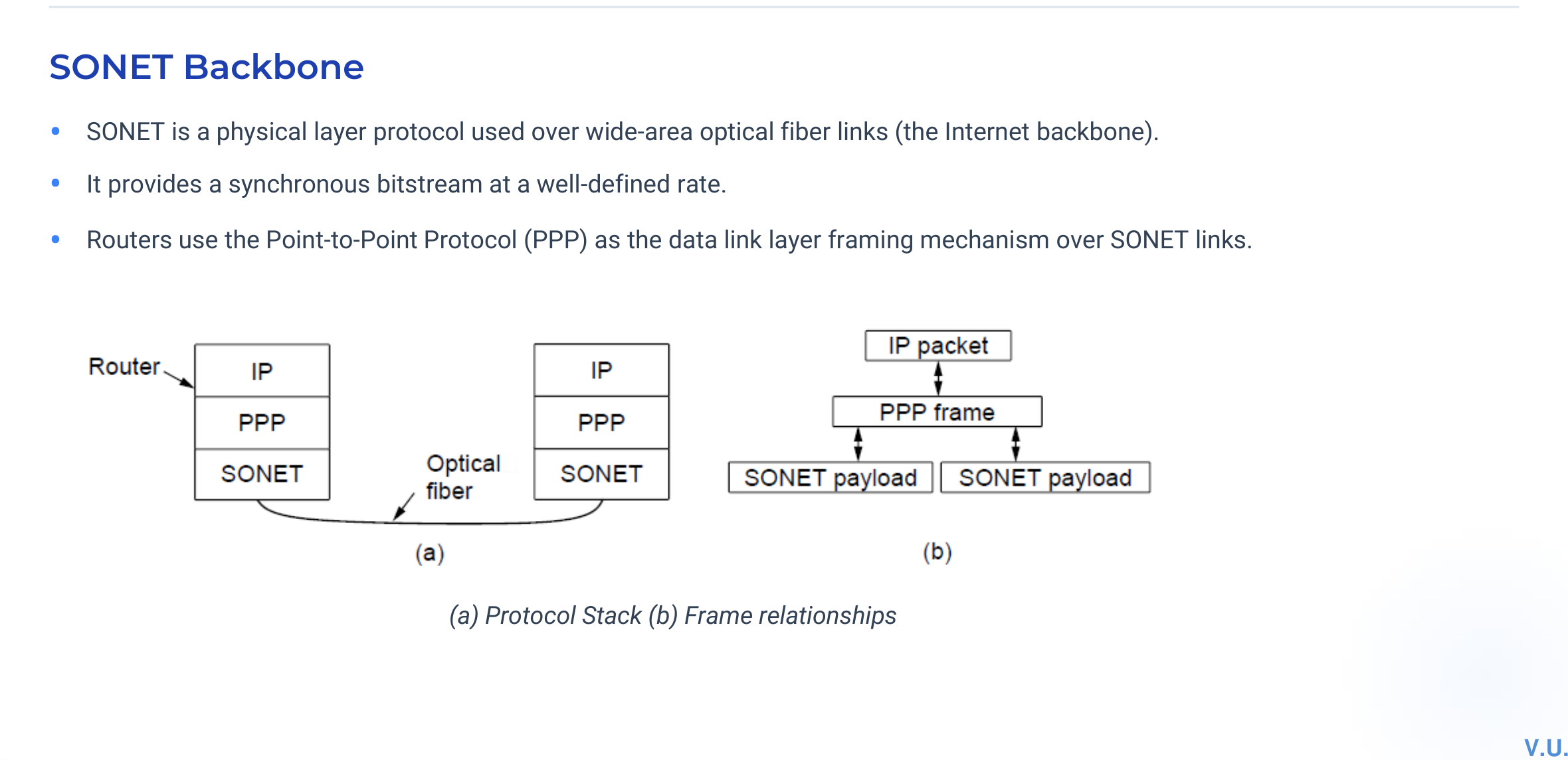
SONET is a synchronous optical transport system used in backbone networks. IP packets can be carried through PPP framing over SONET. The encapsulation path is conceptually IP packet → PPP frame → SONET payload.
Packet over SONET uses PPP as the data-link framing mechanism over an optical transport.
ADSL
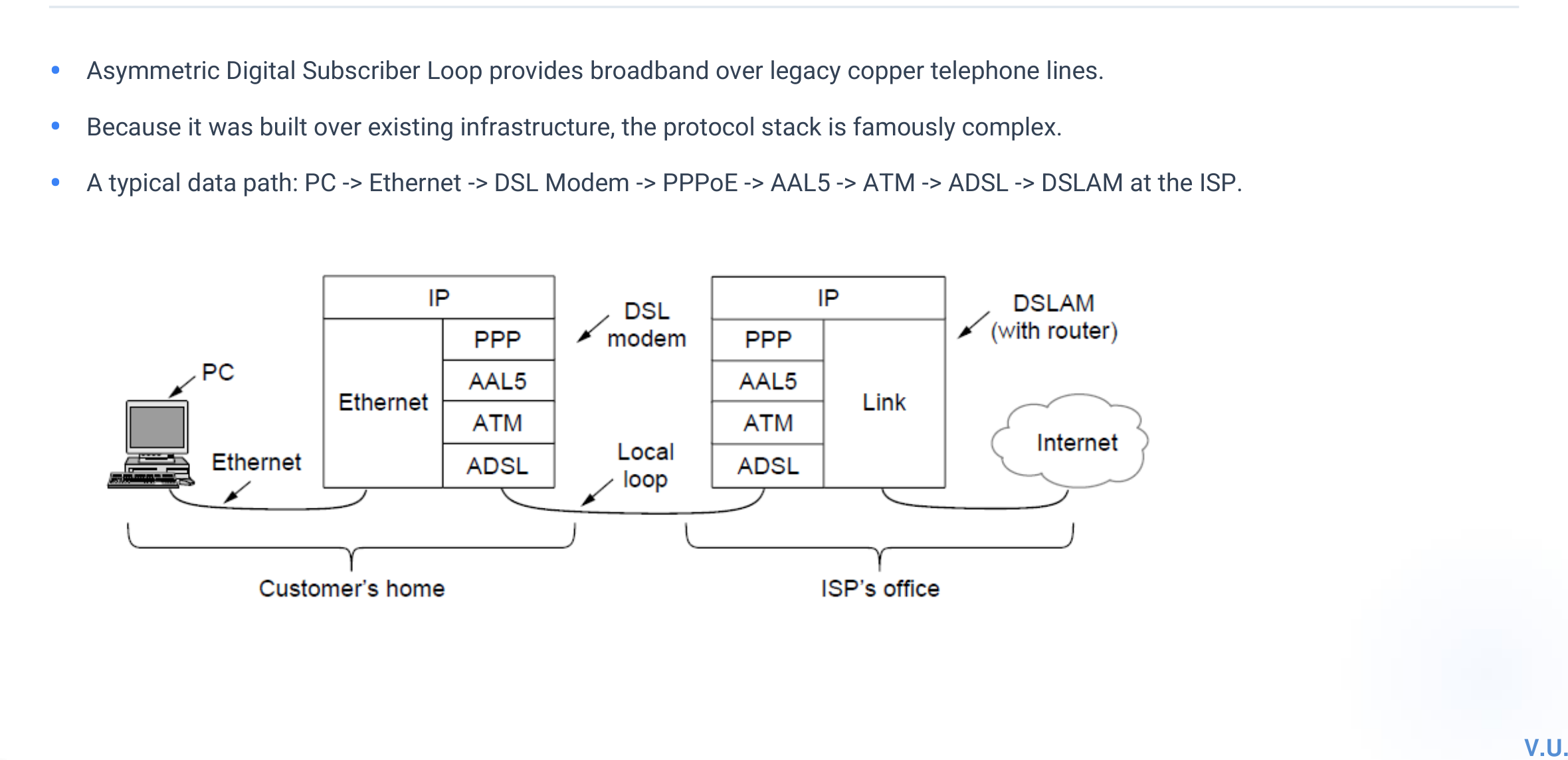
Asymmetric Digital Subscriber Line uses existing telephone copper to provide a higher downstream rate than upstream rate. A typical path is PC → Ethernet → DSL modem → local loop → DSLAM at the provider → ISP network. ADSL systems may carry PPP over ATM/AAL5 in the architecture shown in the lecture.
ADSL access network showing the customer premises, copper local loop, DSLAM, and ISP.
Quick revision
Packet over SONET carries IP/PPP over an optical backbone.
ADSL is asymmetric and reuses telephone copper.
DSLAM aggregates subscriber lines at the provider side.
How multiple stations share one broadcast medium, avoid or resolve collisions, and implement Ethernet.
4.1
Channel Allocation Problem
When many stations share one broadcast channel, the MAC sublayer decides who may transmit. If two stations transmit at an interfering time, a collision can destroy useful work.
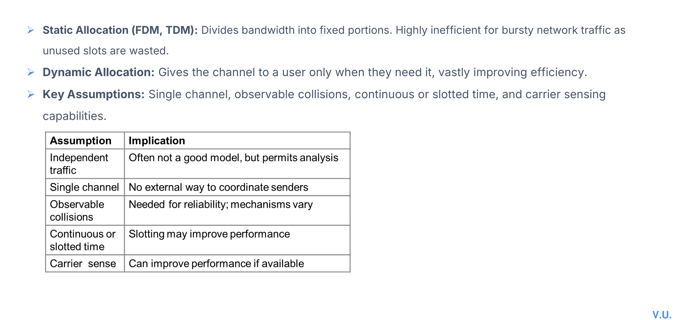
Static allocation reserves capacity; dynamic allocation assigns it when stations actually have traffic.
Allocation
How it works
Strength
Weakness
Fixed / static
Partition channel by frequency, time, code, or fixed ownership
Predictable; no contention after assignment
Idle users waste reserved capacity; inefficient for bursty traffic
Dynamic
Stations contend or coordinate when they have frames
Adapts to bursty demand
Requires collision handling, reservation, or scheduling
Assumptions used to analyse dynamic protocols
Independent stations generate frames.
One shared channel is available.
Collisions are observable or inferable.
Time may be continuous or slotted.
Carrier sensing may be present or absent.
Worked derivation: fraction of slots wasted by collisions
With n hosts, each transmitting in a slot with probability p:
Probability exactly one specified host succeeds: p(1−p)n−1.
Probability exactly one of n hosts succeeds: np(1−p)n−1.
Probability no host transmits: (1−p)n.
Collision fraction: 1 − np(1−p)n−1 − (1−p)n.
Source: CN_Numericals_MAC_Layer.pdf.
Quick revision
Static allocation suits stable demand.
Dynamic allocation suits bursty demand.
A MAC protocol coordinates access to a shared channel.
4.2
ALOHA: Pure and Slotted
ALOHA is a random-access protocol: a station transmits when it has a frame and retransmits after a random delay if a collision is inferred.
Pure ALOHA
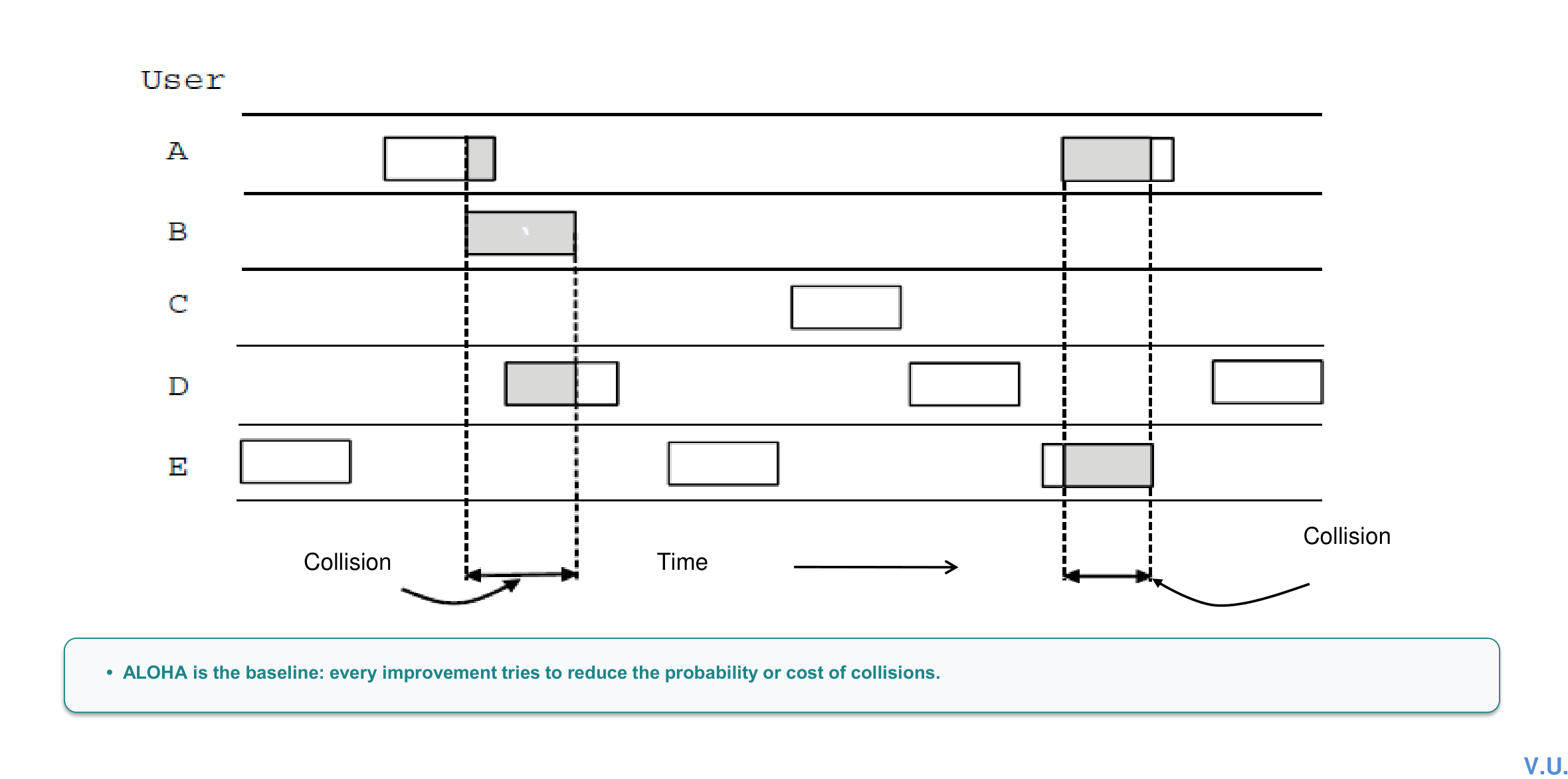
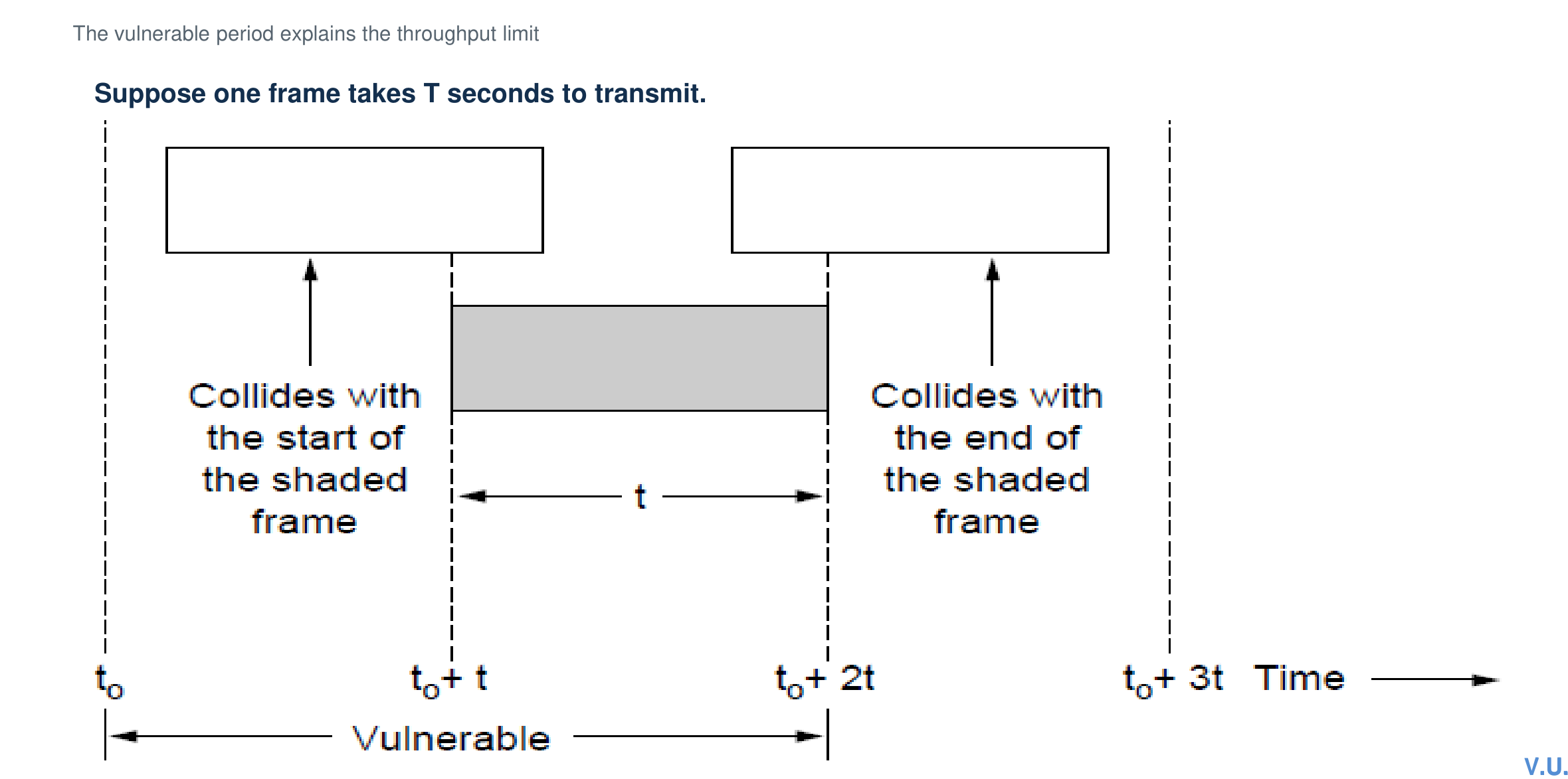
Transmission may begin at any time. A frame of duration T is vulnerable to another frame beginning during the interval from T before its start to T after its start, so the vulnerable period is 2T.
Pure ALOHA permits arbitrary start times.A pure-ALOHA frame is vulnerable for 2T.
Slotted ALOHA
Time is divided into slots of one frame duration and transmission begins only at a slot boundary. Synchronization reduces the vulnerable period to T, improving maximum throughput.
Throughput
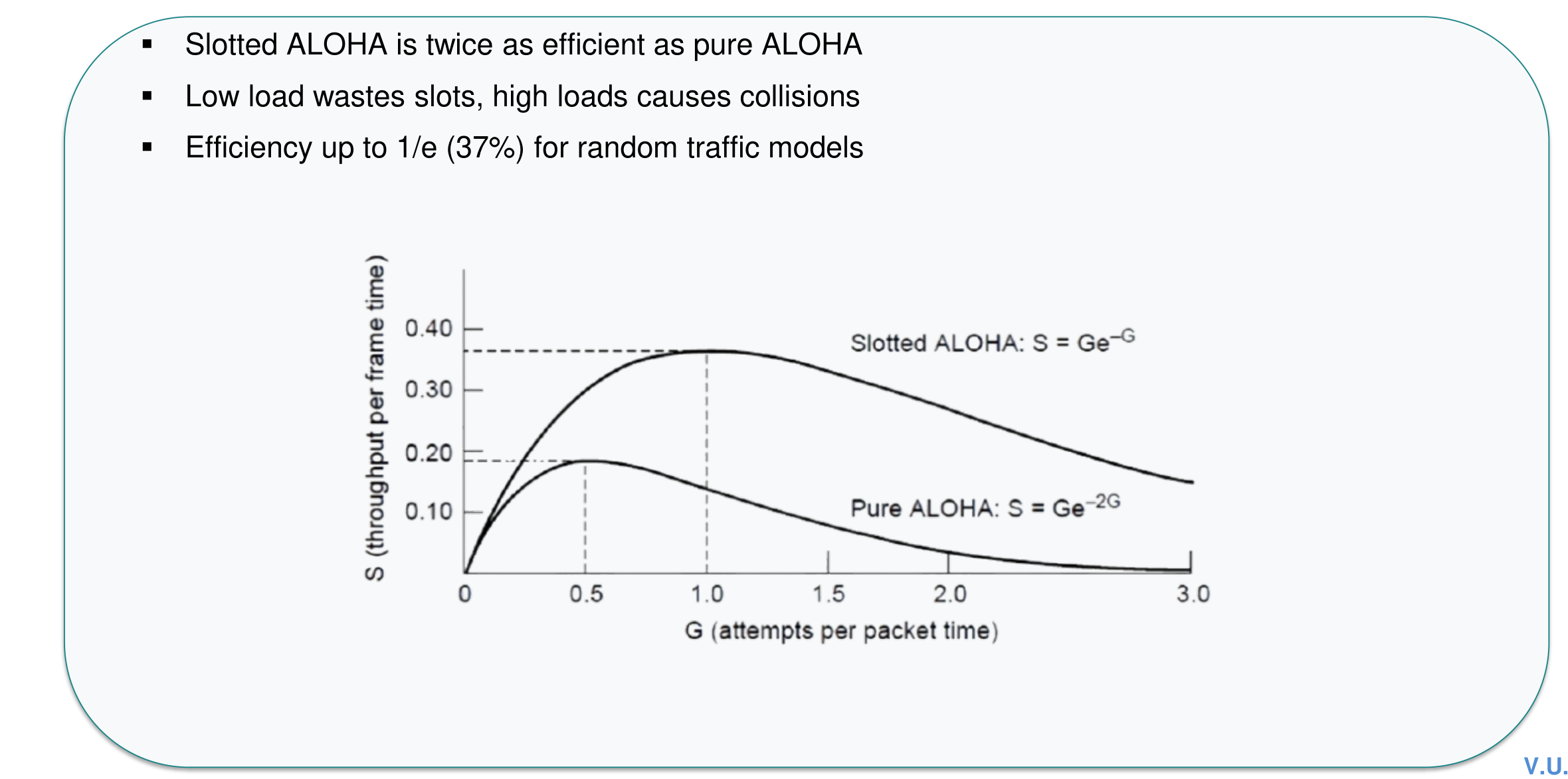
Pure ALOHA: S = G e−2G, maximum 1/(2e) ≈ 18.4% at G = 0.5.
Slotted ALOHA: S = G e−G, maximum 1/e ≈ 36.8% at G = 1.
Slotted ALOHA doubles the theoretical peak throughput by halving the vulnerable period.
Worked numerical: slotted ALOHA success
Problem: 50 requests/s are generated; slot duration is 40 ms. Find first-attempt success and exactly k collisions followed by success.
Offered load: 25 slots/s, so G = 50/25 = 2 attempts/slot.
Success in a slot: e−G = e−2 ≈ 0.1353.
Exactly k collisions then success: (1 − e−2)ke−2 ≈ 0.1353(0.8647)k.
Verified against CN_Numericals_MAC_Layer.pdf and Tutorial 3.
Common mistake
Do not swap the exponents: Pure ALOHA uses e−2G; Slotted ALOHA uses e−G.
Quick revision
Pure ALOHA transmits immediately; Slotted ALOHA waits for slot boundaries.
Vulnerable periods: 2T and T.
Peak throughputs: 18.4% and 36.8%.
4.3
CSMA/CD
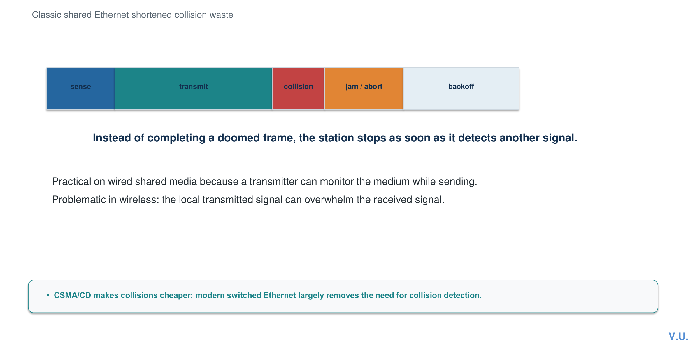
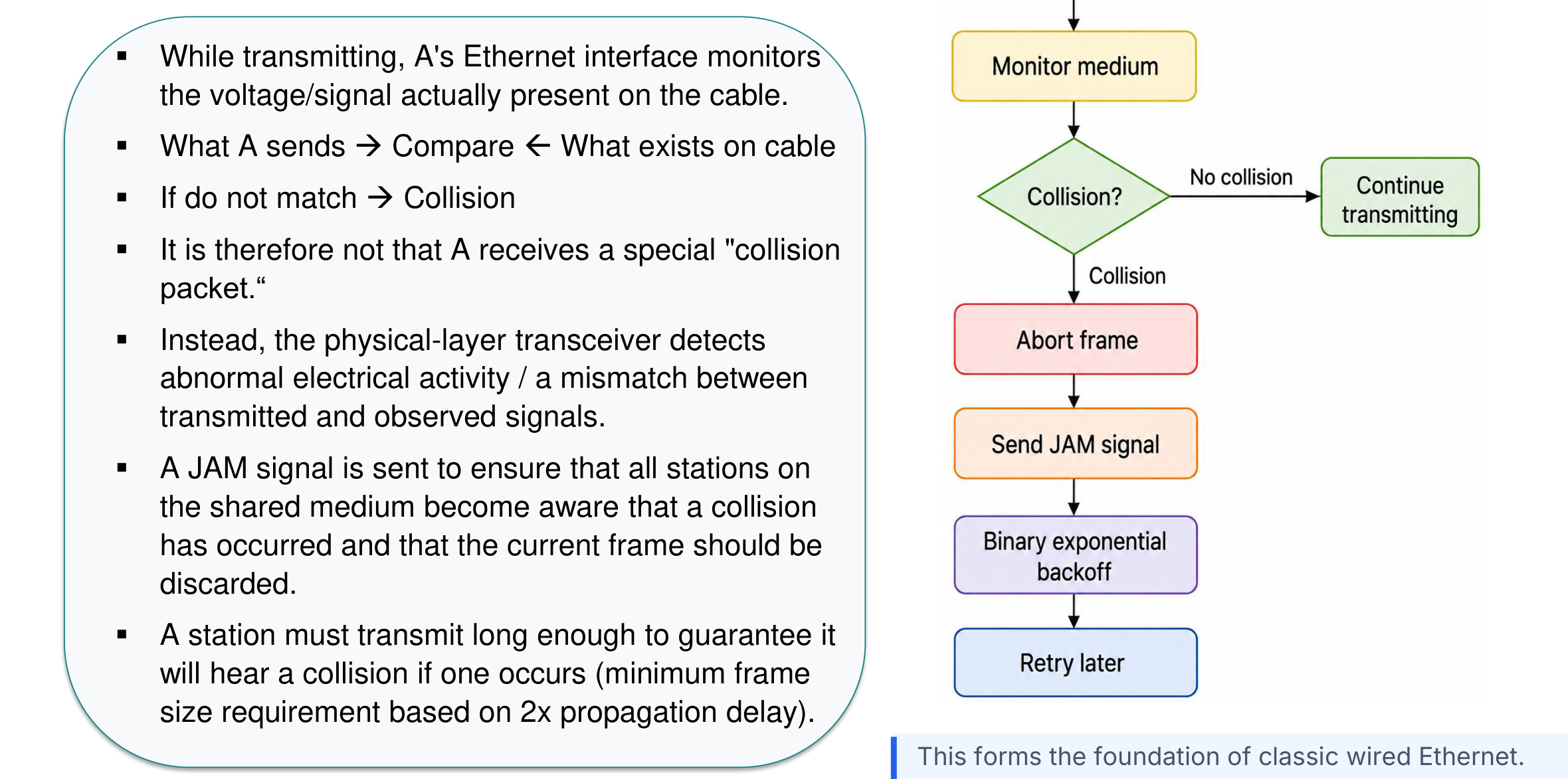
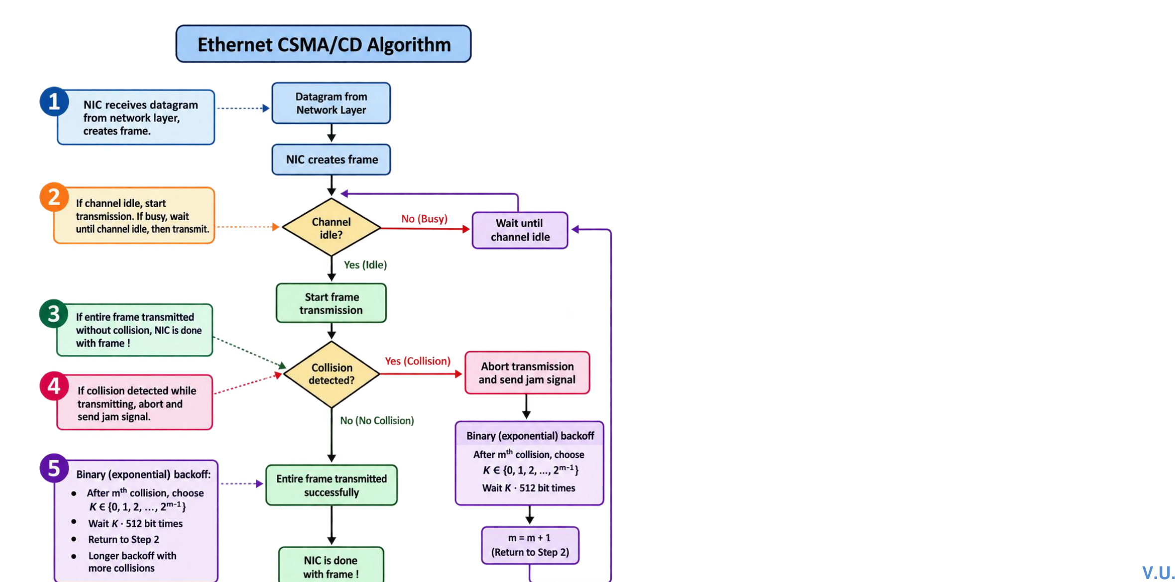
Carrier Sense Multiple Access listens before sending. Collision Detection adds the ability to monitor the medium while transmitting, abort when a collision is detected, send a jam signal, and retry after binary exponential backoff.
CSMA/CD shortens wasted time by aborting a collided frame rather than finishing it.
Sense the channel.
If idle, transmit; if busy, defer according to the persistence rule.
Continue listening while transmitting.
On collision, abort and send a jam signal.
Choose a random backoff interval from a range that grows after repeated collisions.
Retry until success or the attempt limit is reached.
Classic shared Ethernet CSMA/CD decision flow.
Why the minimum frame length exists
The sender must still be transmitting when a worst-case collision propagates back from the farthest station. Therefore frame transmission time must be at least the round-trip propagation time: L/R ≥ 2Tprop, or Lmin = 2RTprop.
Minimum frame time must cover round-trip propagation.
4.4
Collision-Free Protocol: Bit Map
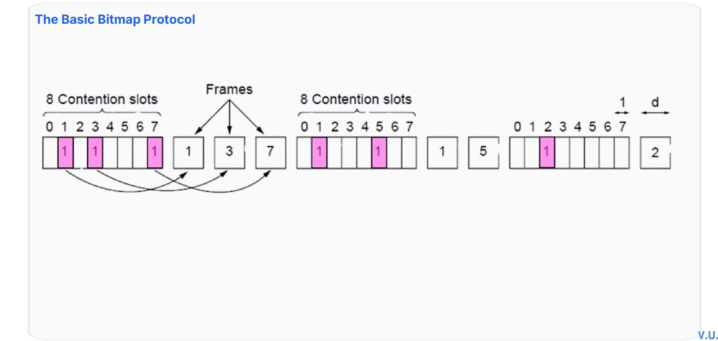
In the basic bit-map protocol, a contention period contains one reservation bit per station. Station i sets bit i if it has a frame. After the reservation phase, ready stations transmit in numerical order without collisions.
Reservations consume N bit slots; the following data phase is collision-free.
Performance intuition
At high load, reservation overhead is shared across many transmitted frames.
At low load, scanning N reservation bits for only a few frames creates significant delay.
The protocol is fair by station order but higher-numbered stations may wait longer.
Worked derivation: worst-case waiting
If all N stations have frames of d bit times and the highest-numbered station becomes ready just after its reservation bit passes, it waits for:
(N−1)d bit times for other frames in the current round,
N reservation bit times for the next bitmap,
(N−1)d bit times before its turn in the next data phase.
Worst-case wait: N + 2(N−1)d bit times.
Quick revision
One reservation bit belongs to each station.
No collisions occur in the data phase.
High-load efficiency is better than low-load efficiency.
4.5
Collision-Free Protocol: Token Ring
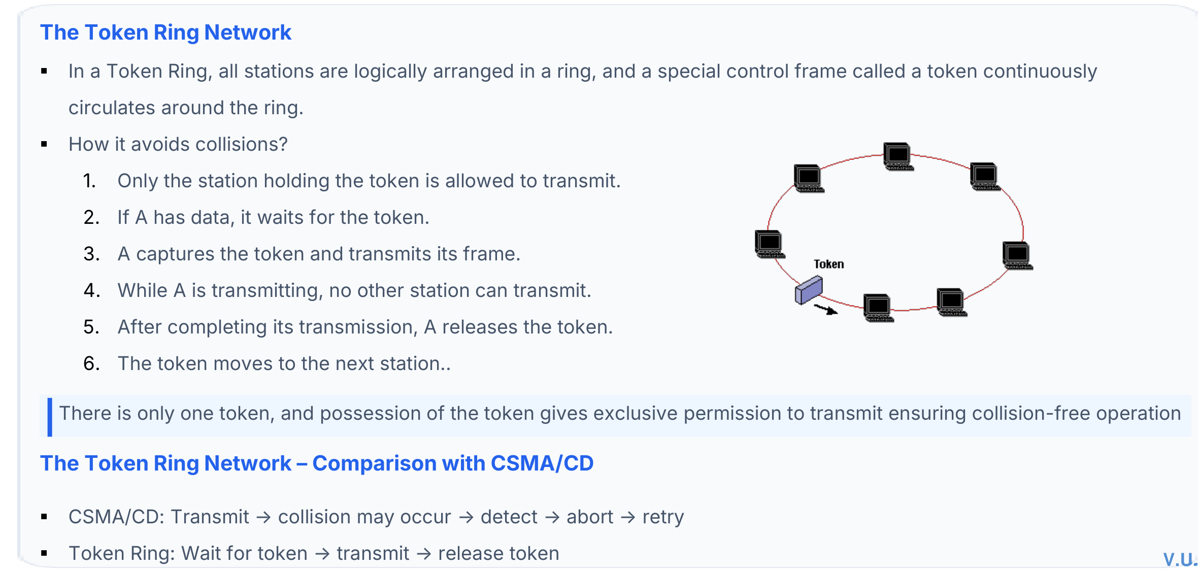
Stations are logically arranged in a ring. A special control frame called a token circulates. Only the station holding the token may transmit, so simultaneous transmissions do not collide.
Exclusive possession of the token grants temporary permission to transmit.
Operation
A station with no frame passes the token.
A station with data captures the token and sends within the token-holding limit.
After completing transmission, it releases a new token.
Monitoring procedures recover from a lost token or duplicate tokens.
Practice numerical: token holding time
Problem: A 4 Mbit/s token ring permits a token holding time of 10 ms. What is the longest frame?
Token passing is deterministic and collision-free.
Token loss and station failure require recovery mechanisms.
4.6
Collision-Free Protocol: Binary Countdown
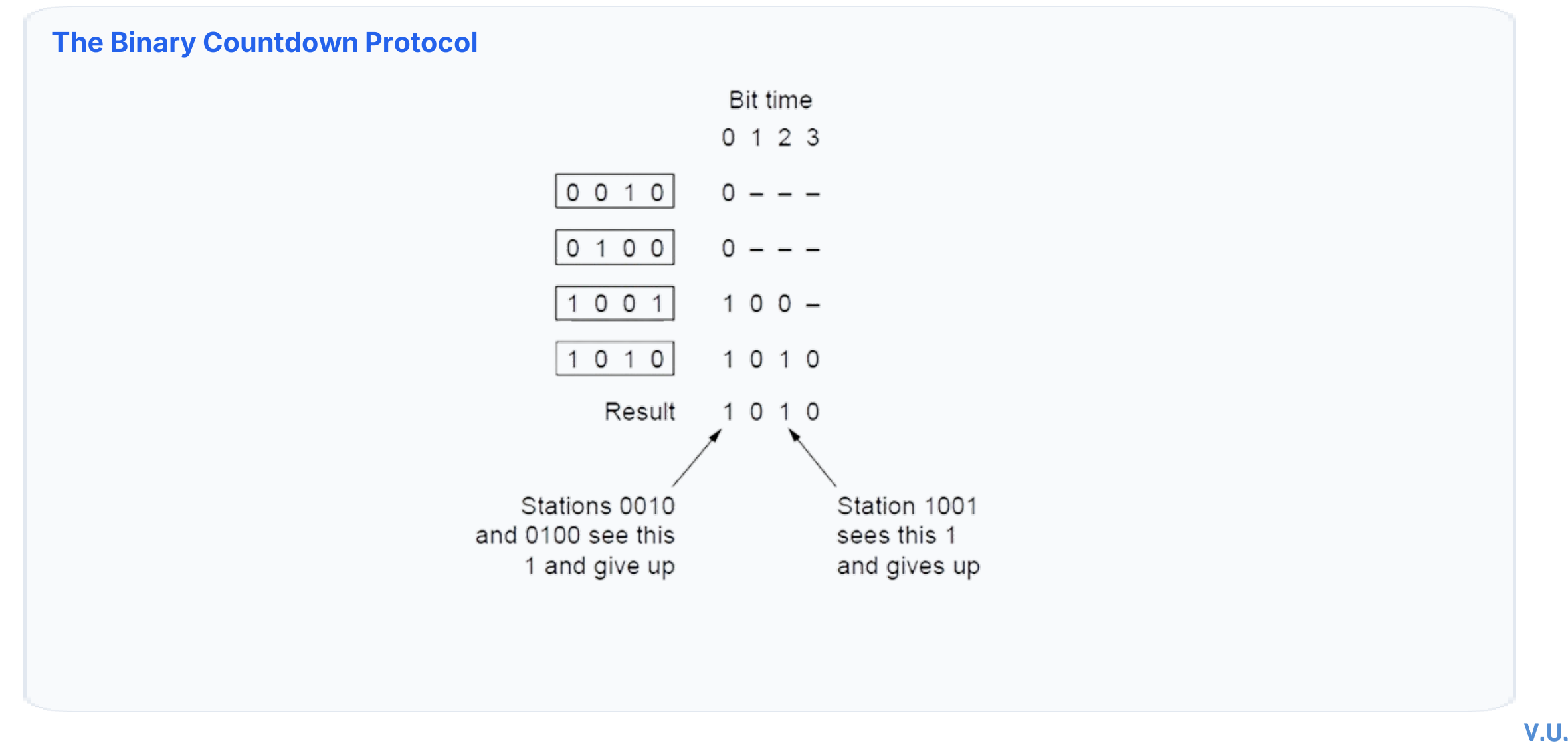
Ready stations transmit their binary addresses one bit at a time, usually from the most significant bit. A dominant bit value overwrites the other value on the shared channel. A station that observes a higher-priority bit withdraws; the highest address remains and transmits.
Bitwise arbitration resolves contention without destroying the winner's transmission opportunity.
Priority is deterministic, so fixed addresses can starve low-priority stations.
Rotating or virtual priorities can improve fairness.
Quick revision
Stations arbitrate using address bits.
The dominant address wins without a destructive collision.
Efficiency is good, but fairness needs attention.
4.7
Limited Contention Protocols and Adaptive Tree Walk
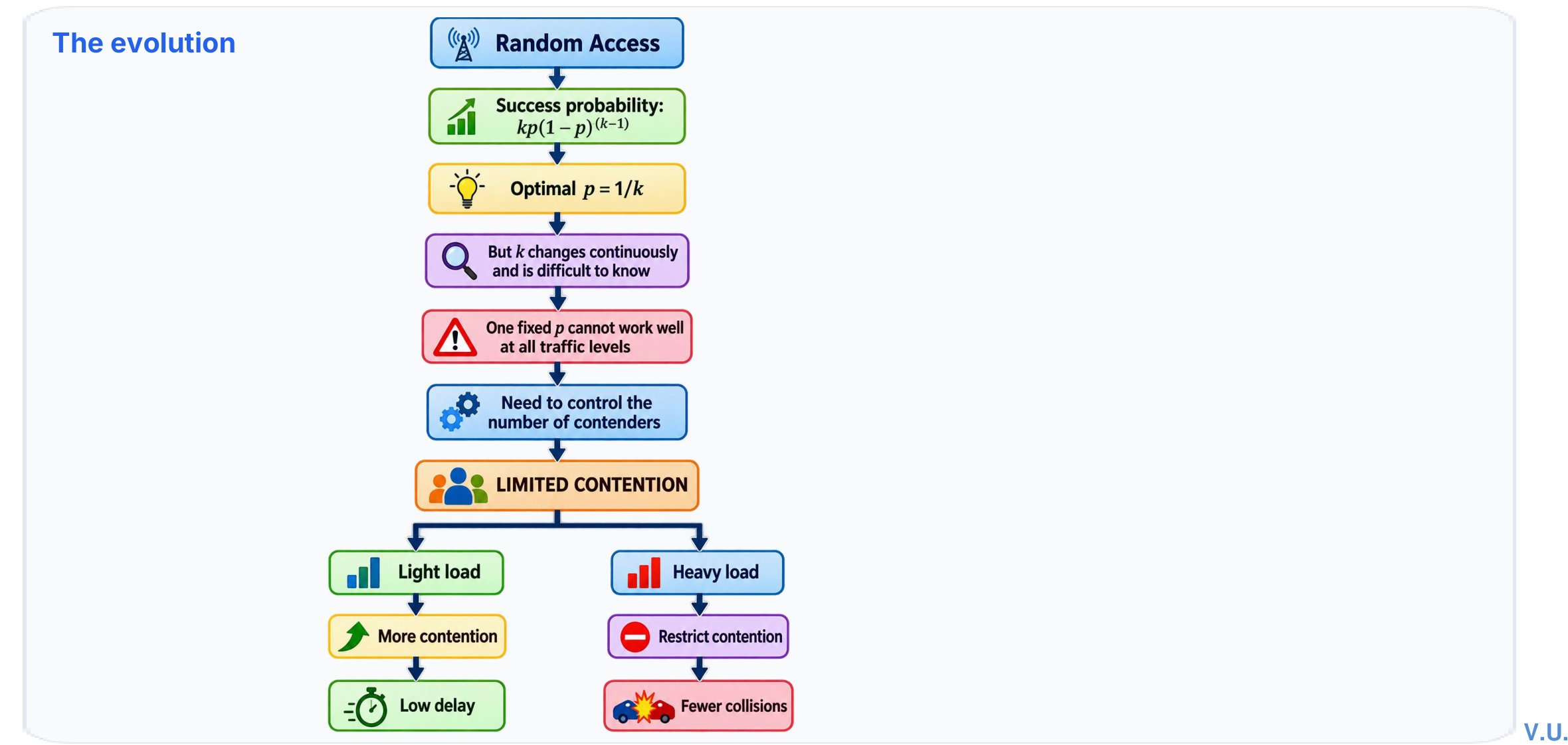
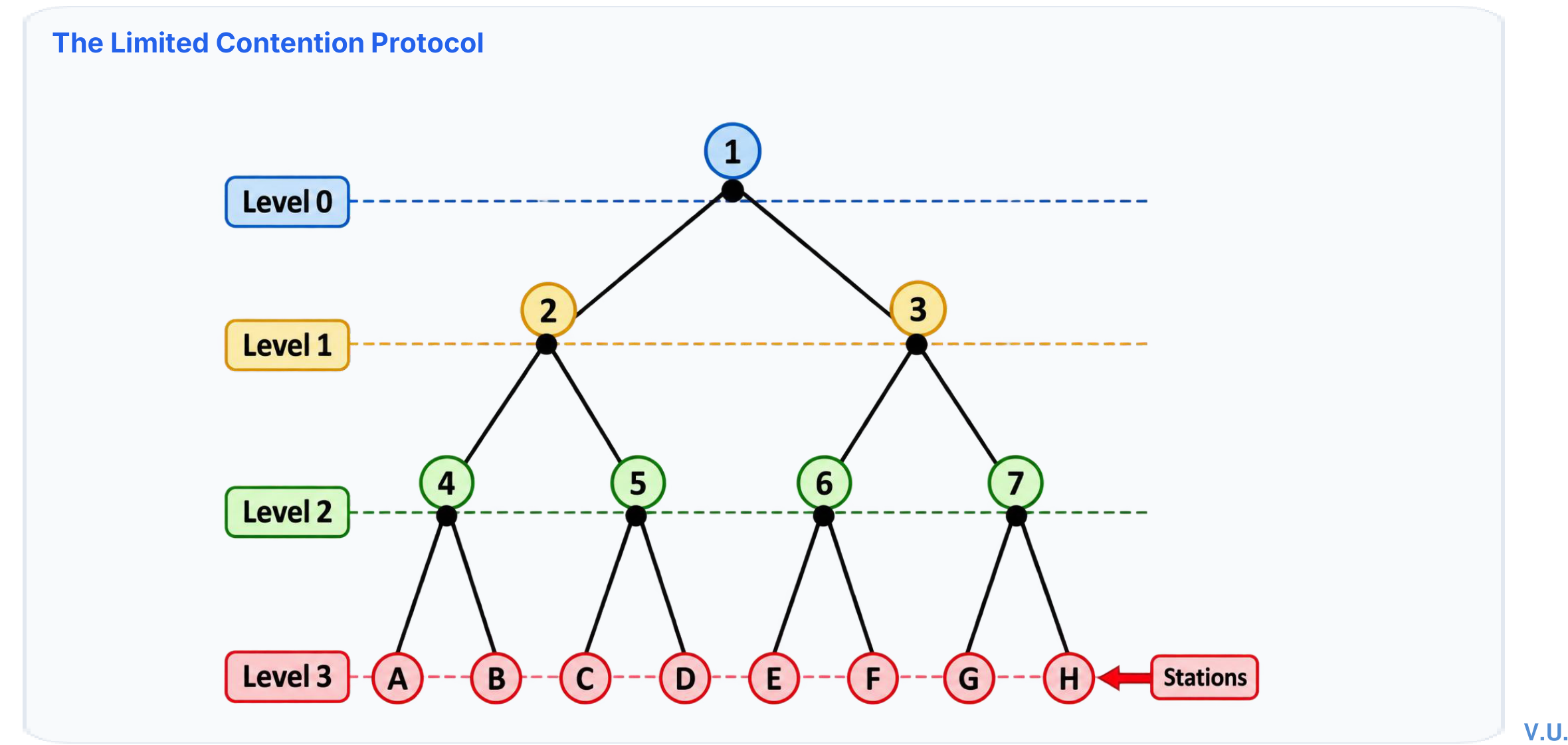
Contention protocols perform well at low load because a station can transmit quickly. Collision-free protocols perform well at high load because they schedule access. Limited-contention protocols adapt between these extremes.
Protocol choice balances low-load delay against high-load collision overhead.
Adaptive tree walk
Stations correspond to leaves of a binary tree. A contention slot tests a node representing a group of stations. No transmission means the group is empty; one transmission succeeds; a collision causes the algorithm to test the node's child groups. Group size can be chosen according to load.
Colliding groups are recursively split until individual ready stations are isolated.
Worked example: prime-numbered stations
Stations 2, 3, 5, 7, 11, and 13 among 1–16 become ready. Following the supplied tree traversal, the contention groups tested are:
Verified against CN_Numericals_MAC_Layer.pdf and Tutorial 4.
Quick revision
Limited contention mixes random access with structured reservation.
Adaptive tree walk splits only groups that collide.
It adjusts the collision group size to load.
4.8
Classic Ethernet (IEEE 802.3)
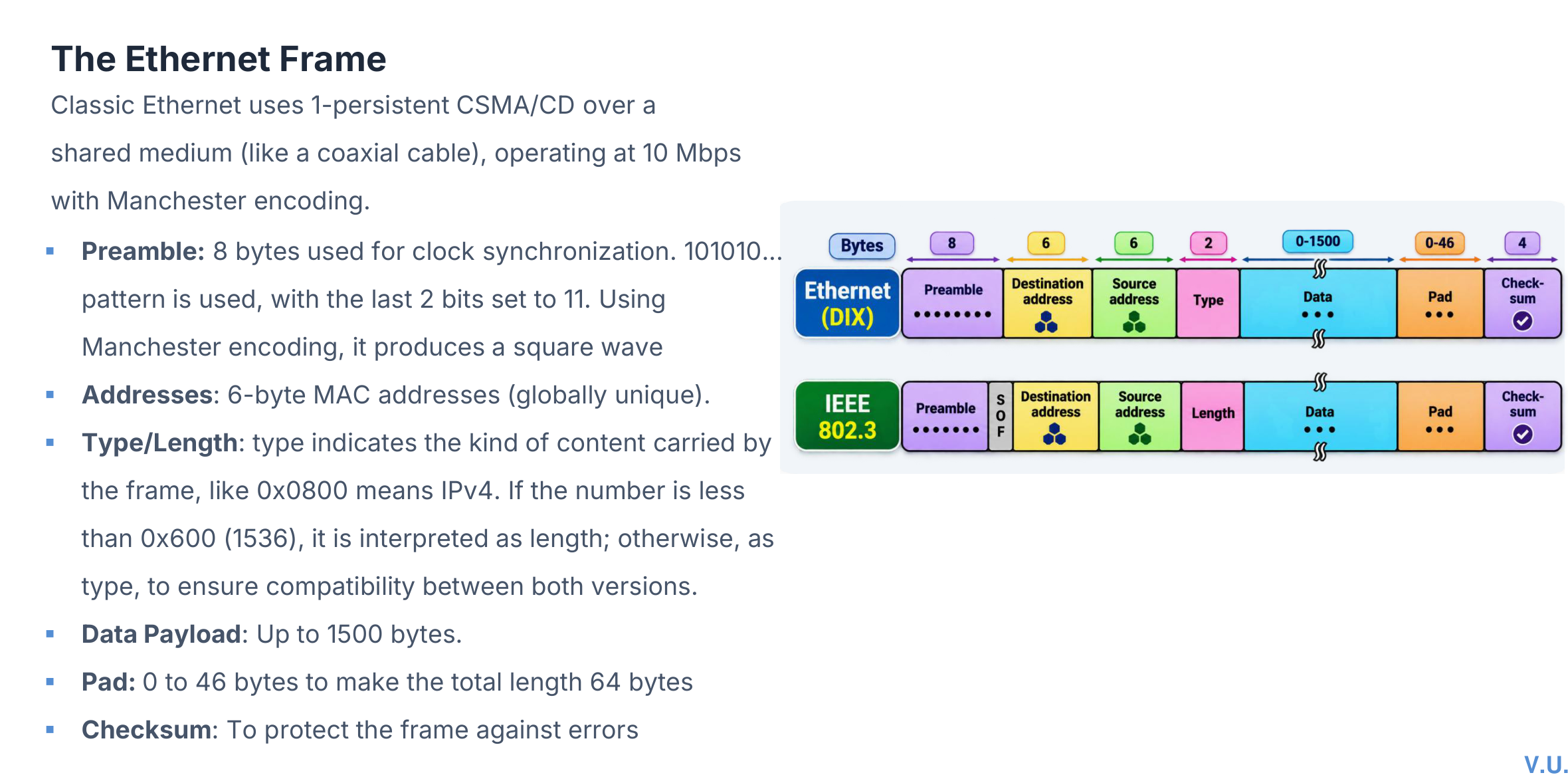
Classic Ethernet used a shared coaxial cable or hubs, Manchester encoding at 10 Mbit/s, and 1-persistent CSMA/CD. Every station in the collision domain saw the shared signal.
Ethernet frame fields and their sizes.
Field
Size
Purpose
Preamble + SFD
8 bytes
Clock synchronization and start delimiter
Destination address
6 bytes
Intended receiver or group
Source address
6 bytes
Sender
Type/Length
2 bytes
Upper-layer type or payload length
Payload
46–1500 bytes
Carried data
Pad
0–46 bytes
Ensures minimum frame length
FCS/CRC
4 bytes
Error detection
The frame from destination address through FCS is at least 64 bytes and at most 1518 bytes without VLAN tagging. The minimum keeps a CSMA/CD sender active long enough to detect a worst-case collision.
Classic shared Ethernet combines frame rules with the CSMA/CD access algorithm.
Worked example: is padding required?
An IP packet is 60 bytes. Without LLC, Ethernet adds destination (6), source (6), type/length (2), and FCS (4): 18 bytes.
Total: 60 + 18 = 78 bytes.
Final answer: No padding is needed because 78 bytes exceeds the 64-byte minimum.
Source: CN_Numericals_MAC_Layer.pdf and Tutorial 4.
Exam focus
Draw and label the Ethernet frame, state the 64-byte minimum and 1518-byte standard maximum, and relate the minimum to collision detection.
Quick revision
Classic Ethernet is a shared collision-domain system.
It uses CSMA/CD and a 64-byte minimum frame.
Payload is 46–1500 bytes.
4.9
Switched, Fast, and Gigabit Ethernet
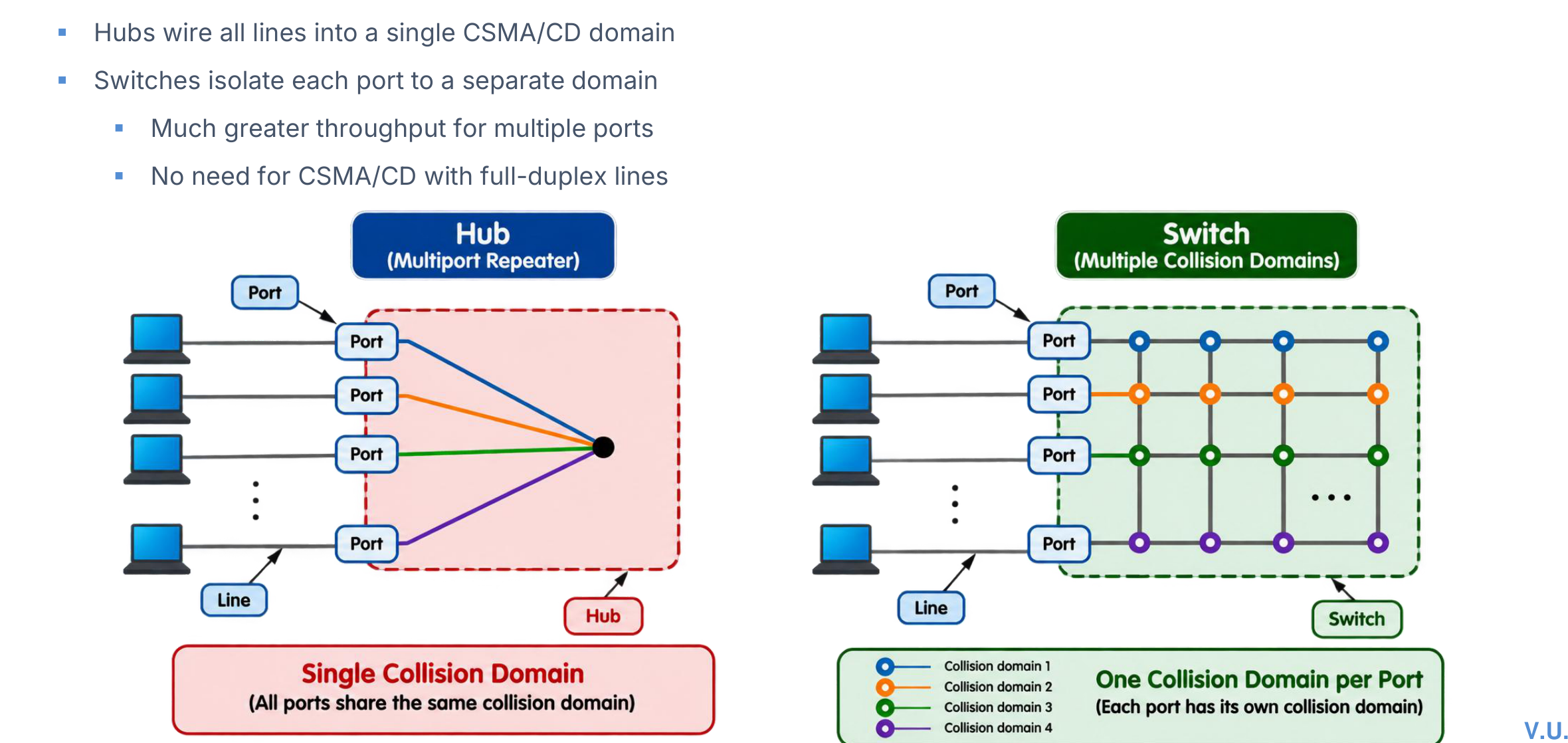
A hub repeats signals into one shared collision domain. A switch learns MAC addresses and forwards frames only toward the appropriate port, giving each full-duplex link its own collision domain. Full-duplex switched Ethernet does not need CSMA/CD.
Switching separates collision domains and permits simultaneous full-duplex conversations.
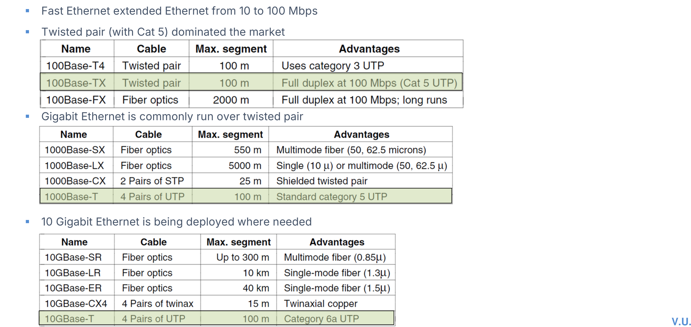
Representative Fast and Gigabit Ethernet physical variants from the lecture.
Concept numerical: faster Ethernet and collision detection
If a network transmits 10 times faster but keeps the same minimum frame size, its frame finishes 10 times sooner. To preserve collision detection, the maximum round-trip propagation time must also be about 10 times smaller.
Conclusion: reduce the maximum shared-cable diameter (or repeater path) roughly in proportion to the speed increase. Modern switched full-duplex links remove collisions entirely.
Quick revision
Switch: one collision domain per port; hub: one shared collision domain.
Fast and Gigabit Ethernet preserve the Ethernet frame format.
Full-duplex switched Ethernet does not use CSMA/CD.